WANG Haiyan, GUO Xinyu, LIU Zhe, *, and GAO Huiwang



A Comparative Study of CART and PTM for Modelling Water Age

WANG Haiyan1), GUO Xinyu2), LIU Zhe1), *, and GAO Huiwang1)

1),,,266100,2),,790-8577,

CART (Constituent-oriented age and residence time theory) and PTM (Particle-tracking method) are two widely used numerical methods to calculate water age. These two methods are essentially equivalent in theory but their results may be different in practice. The difference of the two methods was evaluated by applying them to calculate water age in an idealized one-dimensional domain. The model results by the two methods are consistent with each other in the case with either spatially uniform flow field or spatially uniform diffusion coefficient. If we allow the spatial variation in horizontal diffusion, a term called pseudo displacement arising from the spatial variation of diffusion coefficient likely plays an important role for the PTM to obtain accurate water age. In particular, if the water particle is released at a place where the diffusion is not the weakest, the water age calculated by the PTM without pseudo displacement is much larger than that by the CART. This suggests that the pseudo displacement cannot be neglected in the PTM to calculate water age in a realistic ocean. As an example, we present its potential importance in the Bohai Sea where the diffusion coefficient varies spatially and greatly.

CART; PTM; pseudo displacement; water age

1 Introduction

Advection and diffusion are two important processes in coastal material transport. The material transport timescales play an important role in the algal bloom (Hilton, 1998). Because of the complex spatiotemporal structure of coastal currents, it is helpful to define auxiliary variables, such as water age, to understand the material transport processes in coastal zone of oceans (Zimmerman, 1976; Takeoka, 1984; Deleersnijder, 2001; Monsen, 2002; Delhez, 2004). Water age is defined as the time elapsed since the departure of a water particle from an area, where its age is prescribed to be zero, to its arrival at a water body of interest (Bolin and Rodhe, 1973; Takeoka, 1984).

Numerical simulation is one of the major methods for studying water age. Compared with other methods (,field observations and theoretical study), numerical simulation can consider both advection and diffusion processes in a realistic ocean with complex topography and forcing conditions. Therefore, numerical simulation is widely used in calculating mean water age (Chen, 2007; Wang, 2010; Liu, 2011; de Brye, 2013; Liu, 2012). The mean water age is defined as the mass-weighted arithmetic average of the ages of all of the water particles within a target domain.

Among the aforementioned studies on mean water age, constituent-oriented age and residence time theory (CART, www.climate.be/cart) (Deleersnijder, 2001) and par- ticle-tracking method (PTM) (Zhang, 1995) are two widely used methods. For instance, Wang(2010) studied the mean age of Changjiang River water and de Brye(2013) studied the mean age of canal and dock water by the CART; Chen (2007) studied the mean age of Alafia River water and Liu(2011) studied the mean age of the Tahan Stream, Hsintien Stream, and Keelung River water by the PTM; Liu(2012) used both the CART and PTM to investigate the mean age of Yellow River water in the Bohai Sea.

The CART obtains mean water age by solving two Eulerian equations. As a Lagrangian method, the PTM traces water particles along their pathways and records their ages as time passes. These two methods are essentially equivalent in theory (Liu, 2012). However, the mean water age calculated by the CART and PTM may be different in practice (Liu, 2012). In order to propose some useful suggestions for studying mean water age in a realistic ocean with two methods, the difference of the two methods was evaluated by applying them to an idealized one-dimensional channel in this study.

2 Model Description

2.1 CART Model

To calculate mean water age(,,,) using the CART (Deleersnijder, 2001), two equations need to be solved for the concentration(,,,) and age concentration(,,,) of the targeted water particles, respectively. The concentration(,,,) is controlled by Eq. (1).

, (1)

whereis time;,andare three coordinates in space;,andare velocities in,anddirections, respectively;KandKare horizontal and vertical diffusion coefficients, respectively.

The age concentration(,,,) is calculated by Eq. (2).

. (2)

After solving Eqs. (1) and (2), the mean water age(,,,) is calculated as the ratio of(,,,) to(,,,):

2.2 PTM Model

The PTM module (Zhang,1995) used in this study is from estuarine and coastal ocean model coupled with a sediment transport module (ECOMSED) (Blumberg, 2002). The three coordinates (,,) of a particle in this module was controlled by Eq. (4).

where ∆is time step;is random number with zero mean and unit variance.

The second term on right hand side of Eq. (4) represents pseudo displacement arising from spatial variation in diffusion.

For a particle released at time0, its position is given by Eq. (4) and its age is−0. The mean water age (,,,) is the average of all the particles’ ageat location (,,) at time.

2.3 Model Configuration

We considered a one-dimensional finite domain (signed asdirection) with a lengthof 20km. In the PTM and CART, we used the same grid interval∆(=200m) and time step ∆(=10s).

In the one-dimensional domain, the governing Eqs. (1)–(3) in the CART can be simplified to

, (6)

, (7)

whereis the diffusion coefficient.

The initial values of concentration(,) and age concentration(,) were both set to 0 in the whole domain. At the releasing point (=x), the concentration(,)was always set to 1, that is, the water particle was released continuously at=x. The age concentration at=xwas set to 0, resulting in a zero age of water particle at=x(Bolin and Rodhe, 1973; Takeoka, 1984). At the two ends (=0 and=), the concentration(,)and age concentration(,)both were set to 0, indicating that the water particle could not re-enter the model domain.

In the PTM, the Eq. (4) can be simplified as:

To better understand the movement of a particle, the terms,and∆were defined as char-acteristic diffusion displacement ∆Dif, pseudo displacement ∆Pse, andadvection displacement ∆Adv, respectively.

In the PTM, the initial and boundary conditions were the same as those in the CART. In the experiments for temporally varied flow field (Section 3.2.2), 1 particle was released at=xat each time step within the first period of temporally varied velocity (). In other experiments, a total of 1000 particles were released at=xat the first time step. When a particle was released at=x, its age was set to be 0. Subsequently, the particle age was updated at every time step until it reached the end of the domain (=0 or=), where the particle was excluded from the model.

We recorded the positions of all the particles released in the first period of temporally varied velocity during the total time of calculation. It should be pointed out that the period in the numerical experiments for constant velocity (in all Sections except Section 3.2.2) could be considered as ∆. For calculating the mean water age in a steady state, we need not only the pathways of the particles released in the first period, but also those in the second period and succeeding periods. Based on the fact that the velocity field and diffusivity coefficients used for the PTM calculation were repeated at the same time in every period, we assumed that the particles released in the second and succeeding periods have the same pathways as those released in the first period. The only difference is in the ages of the particles. In this manner, we obtained the pathways of the particles released after the second period without additional PTM calculations. This counting method for mean water age has been used for the mean age of Yellow River water in the BohaiSea(Liu, 2012).

We stopped the calculation when the mean water age did not change with time in the CART and PTM and there- fore obtained the mean water age results in a steady state.

To better understand the mean water age distribution in a steady state, the age frequency distribution function was calculated based on the results of the PTM. The age frequency distribution function() is defined by Eq. (9) (Bolin and Rodhe, 1973),,

where,0() is the total number of particles at;() is the total number of the particles whose age is smaller than or equal to an ageat.

To represent the relative mass of water particles between locationand releasing locationxin a steady state,is defined by Eq. (10):

In the CART,*() and*(x) are the concentration atandx, respectively; in the PTM,*() and*(x) are the particle number atandx, respectively.

3 Results

Because advection and diffusion are two important processes controlling material transport in coastal water, we examine the mean water age distribution controlled by them. In previous studies on mean water age by the PTM, the displacement of a particle usually contains only ∆Difand ∆Adv(Chen, 2007; Liu, 2011) but does not contain ∆Pse. Hence, in addition to the comparison of the CART and PTM, we also pay some attention to the difference between the mean water ages calculated by the PTM with and without ∆Pse, respectively.

3.1 Diffusion

3.1.1 Constant and uniform diffusion coefficient

If the model only includes constant and uniform diffusion coefficient without advection, the analytical solution for mean water age can be found in Appendix A in Liu(2012). In this study,x=0.25; the mean water age is given by Eq. (11):

where at≥0.25,*=−0.25,=0.75; at<0.25,*=0.25−,=0.25.

In the case of=20m2s−1, Fig.1a (black line) shows that mean water age is zero atxand increases as a parabolic function to the distance away fromx. The mean water age calculated by the CART and PTM both agrees well with the analytical solution (Fig.1a).

There is one major peak of frequency at approximately 0 in the age frequency distribution function for the area aroundx(,=0.3) (Fig.1b, red line; Fig.1d). This peak corresponds to the young water particles that quickly spread into this area fromx. In addition to these young water particles, we can also identify the presence of old water particles that have an age longer than 5d (Fig.1b, red line), indicating that the water particles return to=0.3from the area outside=0.3. Therefore, the mean water age of about 3d at=0.3(Fig.1a) results from the coexistence of newly released water particles fromxand the returned water particles from the area outside=0.3.

The age frequency distribution function shows a more complex composition of mean water age in the region far away fromx(,=0.7) (Fig.1c, red line) than that in the region aroundx(,=0.3, Fig.1b, red line). There is one major peak of frequency at approximately 10d in the age frequency distribution function at=0.7(Fig.1c, red line; Fig.1d). This peak corresponds to the water particles that directly spread into this area fromx. However, the frequency at approximately 5–20d in the age frequency distribution function at=0.7is not much smaller than that at approximately 10d (Fig.1c, red line). As a result of coexistence of such water particles, the mean water age at=0.7is about 18d (Fig.1a).

Fig.1e is the extension of results at=0.3and=0.7to the whole model domain (,>0.25). At any locationin the model domain, there are both water particles with small age and water particles with large age. The mean water age atis a result of coexistence of all the water particles at(Fig.1a). Similar to the mean water age, the age corresponds to the max. frequency in the age frequency distribution function increases as a parabolic function to the distance away from thex(Fig.1d).

In the above experiments, we also changed the values ofbut the agreement of the mean water age between the CART and PTM was kept. Apparently, the agreement between two methods is independent of.

3.1.2 Spatially varied diffusion coefficient

We used a spatially varied diffusion coefficient controlled by Eq. (12) (Fig.2a):

where,0=20m2s−1,=15m2s−1.

According to Eq. (8), the displacement of a particle contains ∆Dif(Fig. 2b, black line) and ∆Pse(Fig.2b, red line). ∆Pseis smaller than ∆Difin this case (Fig.2b). ∆Pseis positive at>0.5while negative at<0.5(Fig.2b, red line). Therefore, ∆Psehelps the particle move towards to two ends of the channel.

According to Eq. (12), the minimum diffusion coefficient occurs at=0.5(Fig.2a). Fig.3a shows that the mean water age by the PTM with ∆Pseis almost the same as that by the PTM without ∆Psewhen the releasing point is 0.5(x=0.5). Both of them agree well with the mean water age by the CART. The mean water age is zero atxand increases as a parabolic function to the distance away fromx. However, if the releasing point changes to 0.25(x=0.25), the mean water age by the CART agrees well with that by the PTM with ∆Pse, but is much smaller than that by the PTM without ∆Pseat>0.25(Fig.3c). This is consistent with the results reported by Visser (1997) that the PTM with only∆Difcauses the particles to gather in low diffusion regions. As a result, it is difficult for the particles to leave the low diffusion region (=0.5) (Fig.3d, blue line), and the mean water age at>0.25becomes much longer (Fig.3c, blue line) than that calculated by the CART. As ∆Pseis considered in the PTM, it helps the water particles leave the low diffusion region and move towards=0 or=(Fig.3d, red line).

It must be noted that in the case ofx=0.5, the PTM without ∆Psealso gather water particles in the low diffusion region (=0.5) (Fig.3b, blue line). However, in this case ∆Pseis significantly smaller than ∆Dif(Fig.2b) and it is ∆Difthat determines the displacement of water particles. In addition, since=0.5is also the releasing point of water particles, the age there is always set to be zero according to the boundary condition. Therefore, the mean water ages by the PTM with and without ∆Pseare almost the same (Fig.3a).

In the case ofx=0.25, one major peak at approximately 5d can be found in the age frequency distribution function at=0.5(Figs.4a, b). This peak indicates that whether the PTM contains ∆Pseor not, a certain number of water particles spend approximately 5d spreading into this area fromx. However, the frequency at approximately 5d in the age frequency distribution function at=0.5by the PTM without ∆Pseis smaller than that by the PTM with ∆Pse(Fig.4a). On the other hand, the frequency at longer than 30d in the age frequency distribution function at=0.5by the PTM without ∆Pseis larger than that by the PTM with ∆Pse(Fig.4a). This indicates again that in the calculation of PTM without ∆Pse, compared with the calculation of PTM with ∆Pse, it is difficult for the water particles to leave the low diffusion region (=0.5) (Fig.3d, blue line) with a longer mean water age at>0.25(Fig.3c).

Fig.1 The diffusion coefficient is constant and uniform (20m2s−1) and water particle is released at 0.25L (xr=0.25L). (a) Comparison of mean water ages by CART (black line), PTM (red line), and analytical solution. The analytical solution of Eq. (11) is overlapped by CART (black line). (b) Total number (black line, i.e., M(τ, x) in Eq. (9)) and age frequency distribution function (red line, i.e., φ(τ, x) in Eq. (9)) at x=0.3L. The age range (τ) is limited to 60d since the frequency of particles with age longer than 60d is too small to be identified. (c) The same as Fig.1(b), but for x=0.7L. (d) The age corresponds to the maximum of frequency distribution function at x>0.25L. (e) The age frequency distribution function φ(τ, x) (unit: (0.25d)−1) at x>0.25L. The age range (τ) is limited to 20d.

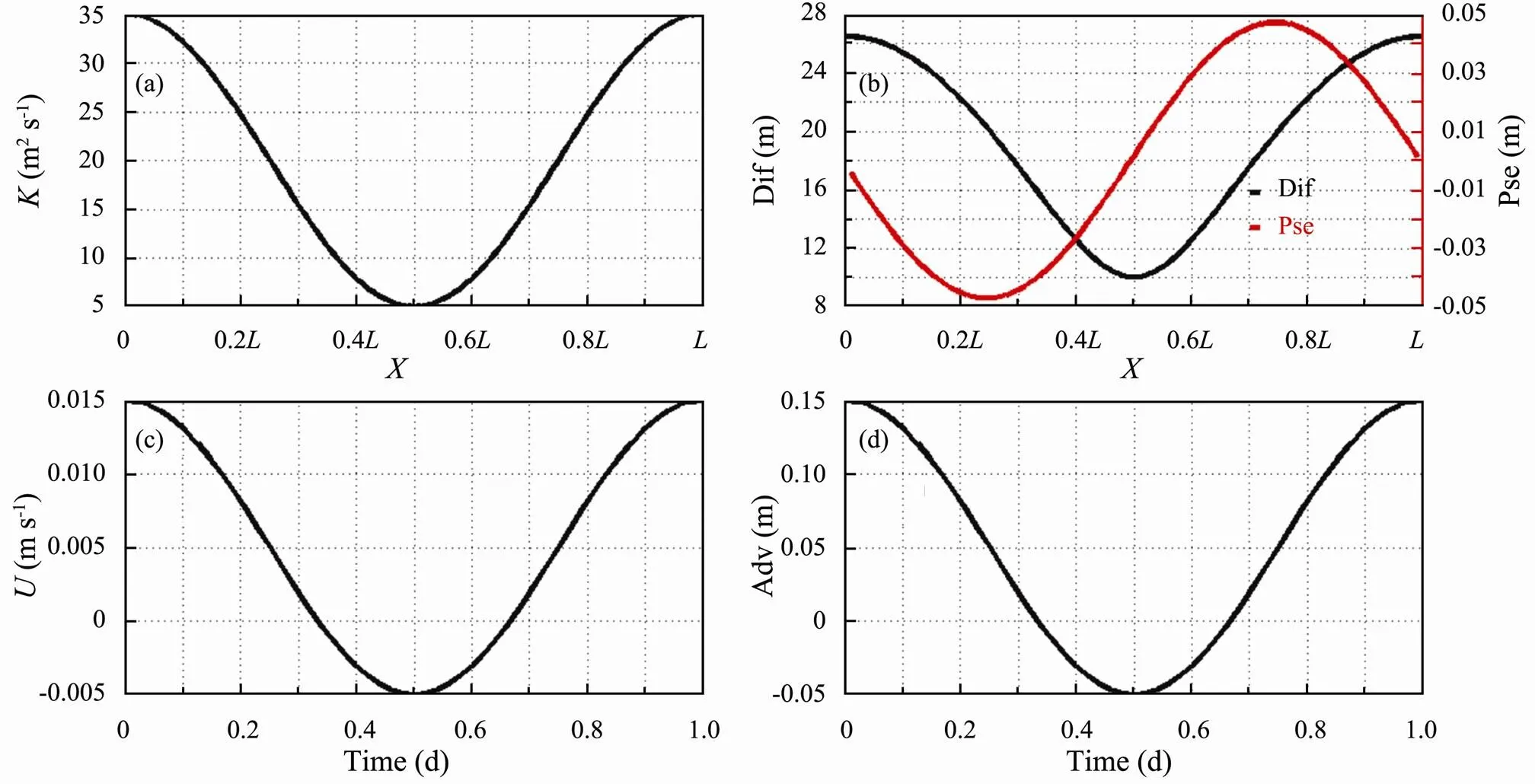
Fig.2 (a) The distribution of spatially varied diffusion coefficient by Eq. (12). (b) Based on the diffusion coefficient shown in Fig.2(a), ∆xDif (black line) and ∆xPse (red line) calculated by Eq. (8). (c) The distribution of temporally varied velocity by Eq. (13). (d) Based on the velocity shown in Fig.2(c), ∆xAdv calculated by Eq. (8). See Section 2.3 for the definitions of ∆xDif, ∆xPse, and ∆xAdv.

Fig.3 The spatially varied diffusion coefficient is controlled by Eq. (12). (a) Water particle is released at 0.5L (xr=0.5L). Comparison of mean water ages by CART (black line), PTM with ∆xPse (red line), and PTM without ∆xPse (blue line). (b) Water particle is released at 0.5L (xr=0.5L). Comparison of R (defined by Eq. (10)) by CART (black line), PTM with ∆xPse (red line), and PTM without ∆xPse (blue line). (c) The same as Fig.3(a), but for xr=0.25L. (d) The same as Fig.3(b), but for xr=0.25L.

Figs.4c and 4d are the extension of results at=0.5to the whole model domain (,>0.25) by the PTM with and without ∆Pse, respectively. At any location, the frequency at small age by the PTM without ∆Pseis smaller than that by the PTM with ∆Pse(Figs.4c and 4d), while the frequency at large age by the PTM without ∆Pseis larger than that by the PTM with ∆Pse(Fig.4c, Fig.4d). As a result, the mean water age by the PTM without ∆Pseis significantly larger than that by the PTM with ∆Pse(Fig.3c). Similar to mean water age, the ages corresponding to the max. frequencies by the PTM with and without ∆Pseboth increase as a parabolic function to the distance away from thex(Fig.4b). The age corresponding to the max. frequency by the PTM without ∆Pseis slightly longer than that by the PTM with ∆Pse(Fig.4b).

In summary, in the case of spatially varied diffusion coefficient, the PTM should include ∆Pse.

Fig.4 The spatially varied diffusion coefficient is controlled by Eq. (12) and water particle is released at 0.25L (xr=0.25L). (a) The age frequency distribution function φ(τ, x) at x=0.5L by PTM with ∆xPse (red line) and by PTM without ∆xPse (blue line). (b) The age corresponds to the maximum of frequency distribution function at x>0.25L by PTM with ∆xPse (red line) and by PTM without ∆xPse (blue line). (c) The age frequency distribution function φ(τ, x) (unit: (0.25d)−1) for x>0.25L by PTM with ∆xPse. (d) The same as Fig.4(c), but for PTM without ∆xPse. The age range (τ) in Figs.4(a), 4(c), and 4(d) is limited to 70d.

3.2 Advection

3.2.1 Constant and uniform velocity

In the case of constant and uniform velocity () without diffusion, the analytical solution for mean water age is/, whereis the distance away fromx. Assuming=0.005ms−1and=0.25, we show the analytical solution in Fig.5a, in which the mean water age is zero atxand increases linearly with the distance away from thex. The mean water age obtained by the CART and PTM agrees well with the analytical solution (Fig.5a). From the age frequency distribution function, each particle’s age equals to the mean age at any locationin the model domain.

3.2.2 Temporally varied velocity

Inthis case, we assumea temporally varied velocity given by Eq. (13) (Fig.2c):

where0=0.005ms−1,=0.01ms−1,=86400s.

According to Eq. (8), in the case of temporally varied velocity without diffusion, the displacement of a particle contains only∆Adv(Fig.2d). Again, we released particles atx=0.25.

Fig.5b shows that the mean water age by the PTM and CART both are zero atxat=105.5d. The mean water age by the PTM increases linearly with the distance away from thexwith a small fluctuation. The mean water age by the CART also increases linearly with the distance away from thexbut with little fluctuation. The PTM deals with each particle and is capable of considering the internal information (, uneven age of particles) inside a grid. The exchange of particles between neighboring grids can be well described in the PTM. However, the uniformity of age of particles within each grid cannot be considered in Eqs. (5)–(6) for CART.

At=105.5d, there is one major peak of frequency at approximately 1.7d in the age frequency distribution function for the area aroundx(,=0.3) (Fig.5c, red line; Fig.5e). This peak corresponds to the young water particles that spread quickly into this area fromx. In addition to these young water particles, we can also identify the presence of old water particles that have an age longer than 2.3d (Fig.5c, red line), indicating that the water particles can return to=0.3from the area outside=0.3because of the negative velocity (Fig.2c). As the case of diffusion, the mean water age (about 2d) at=0.3(Fig.5b) is a result of coexistence of newly released water particles fromxand the returned water particles from the area outside=0.3.

The age frequency distribution function shows a morecomplex composition of mean water age in the region far away fromx(,=0.7) (Fig.5d, red line) than that in the region aroundx(,=0.3, Fig.5c, red line). For instance, there are two major peaks of frequency at approximately 20.6d and 20.9d in the age frequency distribution (Fig.5d, red line). As a result of coexistence of the water particles with different ages, the mean water age at=0.7is about 21d (Fig.5b).

Fig.5f is the extension of results at=0.3and=0.7to the whole model domain (,>0.25). At any locationin the model domain, there are water particles with both small and large ages. The mean water age atis a result of coexistence of all the water particles at(Fig.5b). Compared with the age frequency distribution function under diffusion (Figs.1e, 4c, and 4d), the age of frequency distribution function under advection (Fig.5f) presents a smaller range. Similar to the mean water age, the age cor- responding to the max. frequency in the age frequency distribution function increases linearly with the distance away from thexwith a very small fluctuation (Fig.5e).

In summary, in the case of temporally varied velocity, the mean water age by the PTM and CART agrees well with each other.

Fig.5 Water particle is released at 0.25L (xr=0.25L). (a) The analytical solution for mean water age (x/u, where x is the distance away from xr) with a constant and uniform velocity (0.005ms−1). The mean water ages by CART and PTM overlap with the analytical solution. (b) Comparison of mean water ages by CART (black line) and PTM (red line) with temporally varied velocity controlled by Eq. (13). (c) Total number (black line, M(τ, x)) in Eq. (9) of the particles with ages less than or equal to an age (τ) at x=0.3L; age frequency distribution function (red line, φ(τ, x)) in Eq. (9) at x=0.3L. The age range (τ) is from 1.5 to 3d. (d) The same as Fig.5(c), but for x=0.7L. The age range (τ) is from 20.4 to 21.4d. (e) The age corresponds to the maximum of frequency distribution function at x>0.25L. (f) The age frequency distribution function φ(τ, x) (unit: (0.02d)−1) at x>0.25L. The age range (τ) is limited to 35d. Same as Fig.5(b), the temporally varied velocity is controlled by Eq. (13) in Figs.5(c)–5(f). Figs. 5(b)–5(f) are at time t=105.5d.

4 Discussion

4.1 The Disappearance of the Mean Water Age Difference Between the CART and PTM Without ∆Psein the Case of the Spatially Varied Diffusion Coefficient

The several experiments we discussed above show that the mean water age results by the CART and PTM generally agree well with each other except for that in the case of spatially varied diffusion coefficient (Section 3.1.2). In that case, if the water particle was not released at the place with weakest diffusion, the mean water age by the CART is much smaller than that by the PTM without ∆Pse(Fig.3c). The cause for this inconsistence is because the PTM without ∆Psecollects water particles in low diffusion region (Fig.3d).

From Eq. (12), the average magnitude of gradient of spatially varied diffusion coefficient (, |∂/∂|) is about 3×10−3ms−1at>0.25. In order to calculate the average of |∂/∂| at>0.25, we first calculate the magnitude of gradient of spatially varied diffusion coefficient (|∂/∂|) at each locationat>0.25. The average of |∂/∂| at>0.25is the arithmetic average of all the |∂/∂|at>0.25.

It is of interests to know under what circumstances the phenomenon that the mean water age by the CART is smaller than that by the PTM without ∆Pseat>0.25(Fig.3c) will vanish along with the reduction in |∂/∂|.

We used a spatially varied diffusion coefficient given by Eq. (14) to examine this problem.

By changing value of A in Eq. (14) to 10, 8, 6.5, 5.5, and 5m2s−1, we obtained the average of |∂/∂| as 2×10−3, 1.6×10−3, 1.3×10−3, 1.1×10−3, and 1×10−3ms−1at>0.25, respectively.

Again, we assumedx=0.25. When |∂/∂| decreases, the mean water age difference between the CART and PTM without ∆Pseat>0.25decreases gradually (Fig.6). When the average of |∂/∂| is 1×10−3ms−1, the mean water age by the CART is almost the same as that by the PTM without ∆Pse(Fig.6e). In this case, no matter the PTM includes ∆Pseor not, there is one major peak of frequency at about 5d in the age frequency distribution function at=0.5(Fig.7a), being the same as in the case where the average of |∂/∂| is 3×10−3ms−1(Fig.4a). The frequency at about 5d and longer than 30d by the PTM without ∆Pseat=0.5is almost the same as that by the PTM with ∆Pse(Fig.7a). In the whole domain, the age corresponding to the maximum frequency (Fig.7b) and the age frequency distribution function (Figs.7c, d) by the PTM without ∆Pseis almost the same as that by the PTM with ∆Pse. These features are not found in the results when the average of |∂/∂| is 3×10−3ms−1(Fig.4). There- fore, it is likely that the problem that the mean water age by the CART is smaller than that by the PTM without ∆Pseat>0.25will vanish, if the magnitude of gradient of spatially varied diffusion coefficient decreases to a certain value (, the average of |∂/∂| not larger than 1×10−3ms−1).

On the other hand, advection and diffusion coexist in the realistic ocean. It is therefore necessary to examine the impact of velocity on the PTM without ∆Psein spatially varied diffusion domain. In the next experiments, besides the diffusion coefficient given by Eq. (12), a constant and uniform velocity is added at≥0.25. In Figs.8a, 8b, 8c, and 8d, the velocity is set to 0.0015,0.005, 0.015,and 0.05ms−1, respectively. Again, we assumedx=0.25.

According to Eq. (8), the displacement of a particle contains ∆Dif, ∆Pse, and ∆Advat≥0.25. Here, to show the relative importance of ∆Pseand ∆Adv, a parameter*is defined in Eq. (15):

The average of*equals to 2, 0.67, 0.2, and 0.067 in Figs.8a–8d, respectively. In order to calculate the average of*for>0.25, we first calculate*at each locationfor>0.25. The average of*for>0.25is the arithmetic average of all the*for>0.25.

Fig.6 Water particle is released at 0.25(x=0.25). (a) Comparison of mean water ages by CART (black line), PTM with ∆ (red line), and PTM without ∆ (blue line) with spatially varied diffusion coefficient controlled by Eq. (14) when is set to 10ms. (b)–(e) The same as Fig.6(a), but for spatially varied diffusion coefficient controlled by Eq. (14) when is set to 8, 6.5, 5.5, and 5ms, respectively.

Fig.7 The same as Fig.4, but for spatially varied diffusion coefficient controlled by Eq. (14) when A is set to 5 m2s−1. Water particle is released at 0.25L (xr=0.25L).

Fig.8 Water particle is released at 0.25L (xr=0.25L). (a) Comparison of mean water ages between those by CART (black line), PTM with ∆xPse (red line), and PTM without ∆xPse (blue line). The spatially varied diffusion coefficient is controlled by Eq. (12) and a constant and uniform velocity (0.0015ms−1) is added for x≥0.25L. (b)–(d) The same as Fig.8(a), but the velocities are set to 0.005, 0.015, and 0.05ms−1, respectively.

For*values, the mean water age by the CART agrees well with those calculated by the PTM with ∆Pse(Fig.8, red and black lines). Regarding the PTM without ∆Pse, the agreement is not kept for some values of*. For instance, the mean water age by the CART is much shorter than that by the PTM without ∆Psewhen the average of*is 2 (Fig.8a). In this case, advection is too weak to cover up the mean water age difference caused by spatially varied diffusion coefficient (Fig.3c). In the calculation of the PTM without ∆Pse, it is difficult for water particles to leave the low diffusion region (0.5) and therefore a lot of water particles gather there (Fig.3d).

In the case with both advection and diffusion, even as the average of*decreases to 0.67 (Fig.8b) and 0.2 (Fig.8c), the mean water age by the CART is still shorter than that by the PTM without ∆Pse. However, compared with Fig.8a, the mean water age difference between the CART and PTM without ∆Psegreatly decreases. The mean water age by the CART agrees well with that by the PTM without ∆Psewhen the average of*is 0.067 (Fig.8d). In this case, advection is strong enough to cover up the age difference caused by spatially varied diffusion coefficient. Therefore, if the velocity increases to a certain extent (, the average of*not larger than 0.067), the phenomenon that the mean water age by the CART is shorter than that by the PTM without ∆Pseat>0.25will vanish.

4.2 Application to the Realistic Ocean

In this section, we take the BohaiSeaas an example to study the application of CART and PTM to a realistic ocean. The BohaiSeais a semi-enclosed water body with an average depth of 18m. It is divided into 5 subregions, namely Laizhou Bay, Bohai Bay, Liaodong Bay, the central Basin, and Bohai Strait. The major rivers that flow into the BohaiSeainclude the Yellow River, the Haihe River, the Luanhe River, and the Liaohe River (Fig.9).

The diffusion coefficient and velocity used here were calculated by the model validated by Wang(2008). The horizontal resolution was 1/18 degree in both the zonal and meridional directions. In the vertical direction, 21 sigma levels were distributed (0.000, −0.002, −0.004, −0.010, −0.020, −0.040, −0.060, −0.080, −0.100, −0.120, −0.140, −0.170, −0.200, −0.300, −0.400, −0.500, −0.650, −0.800, −0.900, −0.950, and −1.000). The spatial variability of horizontal diffusion coefficient (1), the ratio of the spatial variability of horizontal diffusion coefficient to the horizontal velocity (2), the spatial variability of vertical diffusion coefficient (3), and the ratio of the spatial variability of vertical diffusion coefficient to the vertical velocity (4) are calculated by Eqs. (16)–(19), respectively:

, (17)

, (18)

We interpolatedKat equal distance in the vertical direction before calculating3and4by Eq. (18) and Eq. (19).

The annualKfor the surface layer of the BohaiSea(Fig.10a) shows that theKis higher in the coastal area (, estuaries, >40m2s−1) than in the offshore area (, the central basin, <20m2s−1). The distribution ofK(Fig.10a) induces a high1in the coastal area (, estuaries, >0.003ms−1) in the surface layer of Bohai Sea (Fig.10c).1is small in the offshore area (, the central basin, about 0.002ms−1) and it is even less than 0.001ms−1in some areas (Fig.10c). Apparently, the magnitude of gra- dient ofspatially varied horizontal diffusion coefficient is smaller in the offshore area than in the coastal area. According to the analysis for the spatially varied diffusion coefficient in Section 3.1.2 and Section 4.1, the∆Psecannot be neglected in the PTM to calculate mean water age when the magnitude of gradient ofspatially varied diffusion coefficientis larger than 0.001ms−1. The2for the surface layer of the Bohai Sea (Fig.10e) shows that2is larger in the coastal area (, estuaries, >0.2) than in the offshore area (, the central basin, <0.2). This indicates that the impact of horizontal advection compared with horizontal diffusion is stronger in the offshore area than in the coastal area. According to the analysis for the spatially varied diffusion coefficient with constant and uniform velocity in Section 4.1, ∆Pseshould be considered in the PTM when*(indicating the effect of diffusion coefficient and velocity in one-dimensional domain) is not less than 0.2. If we consider the effects of both horizontal diffusion coefficient and horizontal velocity in the Bohai Sea, the PTM should include ∆Pseat least for the coastal area (, estuaries) of the Bohai Sea in the horizontal direction.

The annualKalong transect AB in the Bohai Sea (Fig.10b, location being shown in Fig.9) shows that theKis smaller for the surface layer (, shallower than 5m) than in the middle and bottom layers (, deeper than 10m). The distribution ofK(Fig.10b) induces a higher3in the surface layer (, shallower than 5m, >0.003ms−1) than in the middle and bottom layers (, deeper than 10m, about 0.002ms−1) (Fig.10d). In some areas,3is even less than 0.001ms−1(Fig.10d). This indicates that the magnitude of gradient of spatially varied vertical diffusion coefficient is smaller in the middle and bottom area than in the surface area. According to the analysis for the spatially varied diffusion coefficient in Section 3.1.2 and Section 4.1, the∆Psecannot be neglected in the PTM to calculate mean water age when the magnitude of gradient ofspatially varied diffusion coefficientis larger than 0.001ms−1. Fig.10f shows that the4is very large for the whole Bohai Sea (>102) because the vertical velocity is extremely small, indicating that the impact of vertical advection compared with vertical diffusion is very small in the whole Bohai Sea. Hence, it is necessary for the PTM to consider ∆Psein the vertical direction for the whole Bohai Sea.

In summary, the PTM must include ∆Psefor the realistic shallow waters (, the Bohai Sea).

Fig.10 (a) The annual horizontal diffusion coefficient for the surface layer (1 m) of the Bohai Sea. The contour interval is 10m2s−1. (b) The annual vertical diffusion coefficient along transect AB (location is shown in Fig.9). The contour interval is 0.005m2s−1. (c) Based on the horizontal diffusion coefficient shown in Fig.10(a), the spatial variability of horizontal diffusion coefficient (λ1) calculated by Eq. (16). The contour interval is 0.001ms−1. (d) Based on the vertical diffusion coefficient shown in Fig.10(b), the spatial variability of vertical diffusion coefficient (λ3) is calculated by Eq. (18). The contour interval is 0.001ms−1. (e) Based on the horizontal diffusion coefficient shown in Fig.10(a), the ratio of the spatial variability of horizontal diffusion coefficient to the horizontal velocity (λ2) is calculated by Eq. (17). The contour interval is 0.1. (f) Based on the vertical diffusion coefficient shown in Fig.10(b), the ratio of the spatial variability of vertical diffusion coefficient to the vertical velocity (λ4) is calculated by Eq. (19). The contour interval is 0.5. Colors represent the common logarithm of λ4.

5 Summary

The difference in mean water age given by the CART and PTM was studied in an idealized one-dimensional computation domain. The model results by the two methods are consistent with each other in the case with either spatially uniform flow field or spatially uniform diffusion coefficient. In the case with a spatially varied diffusion coefficient, the mean water ages given by the CART and PTM with ∆Pseagree well with each other. If the water particle is released where the diffusion is weakest, the mean water ages given by the CART and PTM without ∆Psealso agree well with each other. If the water particle is released at other places, the mean water age by the CART is much shorter than that by the PTM without ∆Pse. If the magnitude of gradient of spatially varied diffusion coefficient decreases to a certain extent, this difference decreases. The difference also decreases along with the increasing of velocity. As a general conclusion, we recommend that the PTM should include the pseudo displacement caused by the spatial variation in the horizontal and vertical diffusion in a realistic sea area (such as Bohai Sea), especially in the place where the diffusion coefficient varies greatly in space.

Acknowledgements

This work was funded by the National Natural Science Foundation of China (Nos. 41176007 and 40706007). It was carried out while H. Wang was visiting the Center for Marine Environmental Studies at Ehime University, Japan. She thanks the China Scholarship Council (CSC) for supporting her stay in Japan.

Blumberg, A. F., 2002.. HydroQual Inc., Mahwah, New Jersey, 29-31.

Bolin, B., and Rodhe, H., 1973. A note on the concepts of age distribution and transit time in natural reservoirs., 25 (1): 58-62, DOI: 10.1111/j.2153-3490.1973.tb01594.x.

Chen, X., 2007. A laterally averaged two-dimensional trajectory model for estimating transport time scales in the Alafia River estuary, Florida., 75 (3): 358-370, DOI: 10.1016/j.ecss.2007.04.020.

de Brye, B., de Brauwere, A., Gourgue, O., Delhez, E. J. M., and Deleersnijder, E., 2013. Reprint of Water renewal timescales in the Scheldt Estuary., 128: 3-16, DOI: 10.1016/j.jmarsys.2012.03.002.

Deleersnijder, E., Campin, J. M., and Delhez, E. J. M., 2001. The concept of age in marine modelling I. Theory and preliminary model results., 28 (3-4): 229-267, DOI: 10.1016/S0924-7963(01)00026-4.

Delhez, E. J. M., Heemink, A. W., and Deleersnijder, E., 2004. Residence time in a semi-enclosed domain from the solution of an adjoint problem., 61 (4): 691-702, DOI: 10.1016/j.ecss.2004.07.013.

Hilton, A. B. C., McGillivary, D. L., and Adams, E. E., 1998. Residence time of freshwater in Boston’s inner harbor., 124 (2): 82-89, DOI: 10.1061/(ASCE)0733-950x.

Liu, W. C., Chen, W. B., and Hsu, M. H., 2011. Using a three-dimensional particle-tracking model to estimate the residence time and age of water in a tidal estuary., 37 (8): 1148-1161, DOI:10.1016/j.cageo.2010.07.007.

Liu, Z., Wang, H., Guo, X., Wang, Q., and Gao, H., 2012. The age of Yellow River water in Bohai Sea., 117: 1-19, DOI: 10.1029/2012JC008263.

Monsen, N. E., Cloern, J. E., Lucas, L. V., and Monismith, S. G., 2002. A comment on the use of flushing time, residence time, and age as transport time scales., 47 (5): 1545-1553, DOI: 10.4319/lo.2002.47.5.1545.

Takeoka, H., 1984. Fundamental concepts of exchange and transport time scales in a coastal sea., 3 (3): 311-326, DOI: 10.1016/0278-4343(84)90014-1.

Visser, A. W., 1997. Using random walk models to simulate the vertical distribution of particles in a turbulent water column., 158: 275-281, DOI: 10.3354/meps158275.

Wang, Q., Guo, X., and Takeoka, H., 2008. Seasonal variations of the Yellow River plume in Bohai Sea: A model study., 113: 1-14, DOI: 10.1029/2007JC004555.

Wang, Y., Shen, J., and He, Q., 2010. A numerical model study of the transport timescale and change of estuarine circulation due to waterway constructions in the Changjiang Estuary, China., 82 (3): 154-170, DOI: 10.1016/j.jmarsys.2010.04.012.

Zhang, X. Y., 1995. Ocean outfall modeling–Interfacing near and far field models with particle tracking method. PhD thesis. Massachusetts Institute of Technology, Cambridge, 84-109.

Zimmerman, J. T. F., 1976. Mixing and flushing of tidal embayments in the western Dutch Wadden Sea, Part I: Distribution of salinity and calculation of mixing time scales., 10 (4): 149-191, DOI: 10.1016/0077-7579(76)90013-2.

(Edited by Xie Jun)

DOI 10.1007/s11802-015-2393-7

ISSN 1672-5182, 2015 14 (1): 47-58

© Ocean University of China, Science Press and Springer-Verlag Berlin Heidelberg 2015

(May 9, 2013; revised May 30, 2013; accepted November 6, 2014)

* Corresponding author. Tel: 0086-532-66786568 E-mail: zliu@ouc.edu.cn