CAO Pengfei (曹鹏飞) and LUO Xionglin (罗雄麟)**Research Institute of Automation, China University of Petroleum, Beijing 102249, China

Soft Sensor Model Derived from Wiener Model Structure: Modeling and Identification*

CAO Pengfei (曹鹏飞) and LUO Xionglin (罗雄麟)**
Research Institute of Automation, China University of Petroleum, Beijing 102249, China

The processes of building dynamic and static relationships between secondary and primary variables are usually integrated in most of nonlinear dynamic soft sensor models. However, such integration limits the estimation accuracy of soft sensor models. Wiener model effectively describes dynamic and static characteristics of a system with the structure of dynamic and static submodels in cascade. We propose a soft sensor model derived from Wiener model structure, which is an extension of Wiener model. Dynamic and static relationships between secondary and primary variables are built respectively to describe the dynamic and static characteristics of system. The feasibility of this model is verified. Then the expression of discrete model is derived for soft sensor system. Conjugate gradient algorithm is applied to identify the dynamic and static model parameters alternately. Corresponding update method for soft sensor system is also given. Case studies confirm the effectiveness of the proposed model, alternate identification algorithm, and update method.

soft sensor, Wiener model, modeling, alternate identification

1 INTRODUCTION

It is usually difficult to measure the important quality variables, such as oil viscosity, real-time for chemical processes, which brings great difficulty to process control and optimization. Soft sensor technology is an important means to solve this problem [1], which utilizes easily measured variables, such as temperature and pressure, to estimate the quality variables real-time.

The modeling for soft sensor system is the core of soft sensor technology, namely, building the relationship between secondary and primary variables representing easily measured variables and quality variables in chemical processes. The characteristics of a soft sensor system, including dynamic and static components, are described by dynamic and static relationships between secondary and primary variables. Since soft sensor system is nonlinear and always in dynamic state, nonlinear dynamic model is needed for these relationships [2-4]. There are several principal types of nonlinear dynamic modeling methods. Historical values of secondary and primary variables have been used as the inputs of nonlinear model [5, 6], but this modeling method brings in calculation complexity with more model parameters, especially when the soft sensor system has a large number of secondary variables. In order to reduce the calculation complexity, multimodel-based modeling methods are introduced [7, 8], either building the relationship between each secondary and primary variables or describing the system under different working conditions. The feedback network model is also built for soft sensor system [9, 10], but the stability of feedback structure remains to be proved. Although nonlinear dynamic modeling methods are different, most of them add dynamic compensation to nonlinear model in many ways [5-10], and that is integrating the processes of building the dynamic and static relationships between secondary and primary variables, which is one of the major problems. The consequence is that the dynamic and static relationships are compensated by each other. In most cases the parameters and model structure lack physical meaning and the model explanation for soft sensor system may be inappropriate. Although the model may provide accurate estimations for primary variables off-line, neither of the dynamic and static characteristics can be described well, and the generalization ability of models are limited [4, 5, 11]. In order to describe a soft sensor system adequately and estimate quality variable accurately, the two relationships should be built effectively [4, 11, 12].

Static nonlinear relationship may be built more accurately with the sample data obtained when soft sensor system is in steady state [13, 14]. Linear dynamic model, such as transfer function, difference equation, or state space expression, is a good choice for building dynamic relationship, usually through the identification with incremental data of secondary and primary variables at some working point [15, 16]. However, linear dynamic model lacks the description of static nonlinear characteristics. Since a soft sensor system is nonlinear and always in dynamic state, the dynamic and static information is integrated. Therefore, the dynamic and static parts of the measured data cannot be separated to build the dynamic and static relationships between the secondary and primary variables. We need to build these relationships separately with neither the extracted dynamic nor static parts of the measured data but with themselves, andfind some way to combine these relationships to describe the characteristics of soft sensor system and give the estimation for primary variables.

Wiener model is an important block-oriented model, which has been successfully used to represent nonlinear systems in chemical processes, such as distillation and pH neutralization process [17, 18]. Wiener model consists of linear dynamic and static nonlinear submodels in cascade. Based on this structure, Wiener model can effectively describe the dynamic and static nonlinear characteristics of system [19, 20]. Therefore, we propose a soft sensor model derived from Wiener model structure, which presents different expression and is an extension of Wiener model. The model also consists of dynamic and static submodels in cascade. With intermediate variable, the dynamic relationship is built by the dynamic submodel with secondary and intermediate variables, and the static relationship is built by the static submodel with intermediate and primary variables. To reduce the difficulty for parameter identification brought by the model structure [21], the identification is decomposed into two parts based on the hierarchical principle [22]. The dynamic and static submodels are identified based on the conjugate gradient algorithm alternately. The update method for model parameters is also given. Finally, the proposed model is used to estimate pH values in a pH neutralization process and ethylene concentration in a distillation tower real-time, and the model parameters are identified and updated online based on the specific method.

2 PROPOSED MODEL DERIVED FROM WIENER MODEL STRUCTURE

The structure of Wiener model is shown in Fig. 1. The model consists of a linear dynamic submodel N(•) in cascade with a static nonlinear one G(•), and it can effectively describe the dynamic and static nonlinear characteristics of a system [19, 20]. However, there are some shortages: it is more suitable to the process that can be decomposed into fixed dynamic and static parts, with the intermediate variable usually having physical meaning [23-25]; good estimation can be achieved with more samples under comprehensive working conditions and the model remains unchanged online in most cases [25, 26].

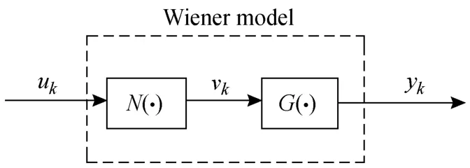
Figure 1 Wiener model structure

In this paper, we build a soft sensor model derived from Wiener model structure. The structure of the proposed model is similar to that of Wiener model, and it is an extension of Wiener model to some extent. The dynamic and static relationships between secondary and primary variables are built by the dynamic and static submodels. The differences from Wiener model are as follows. Firstly, the intermediate variable is constructed without physical meaning and the gain of its dynamic part is designated as 1, so it is suitable to more processes in addition to soft sensor systems. Secondly, the choice for static submodel is more and linear model is chosen and applied in this study. Since soft sensor system is nonlinear and its dynamic and static characteristics may change at different working points, the dynamic and static submodels should be updated online.

We first derive the model for single-input soft sensor system with only one secondary variable and primary variable. In actual processes, soft sensor system has multiple secondary variables, so we extend the model to multi-input soft sensor system. We do not consider delay time, which does not affect the feasibility of the model structure.

2.1 Model for single-input soft sensor system

The dynamic relationship between each secondary and primary variables can be described as below [11, 27].

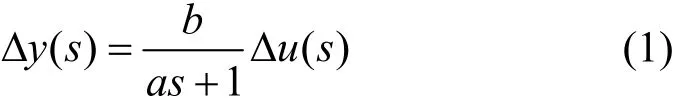
where y is primary variable, u is secondary variable, and (u0, y0) is the steady working point. We have Δy=y−y0and Δu=u−u0, which are the increment of primary and secondary variables. The dynamic relationship is built with Δy and Δu. a and b will change at different working point. In addition to transfer function, the dynamic relationship may be in other forms, such as difference equation, and state space expression, depending on the increments. Actually, we just have u and y but do not know u0and y0, so we could not build the dynamic relationship accurately.

In applications, we prefer a model that eventually gives the estimations for y. Transforming Eq. (1) in the time domain, we have

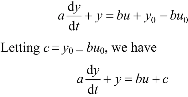
Generally, b and c will change under different working conditions. The static nonlinear relationship could only be built accurately when the system is in steady state, namely d/d0yt=. If d/d0yt≠, the static relationship is inaccurate, since the measured data involves dynamic information.

With /(1)

Δ=Δ+ in the same order of magnitude of u, then yb v

vuas Δ=Δ. With intermediate variable v constructed, we have

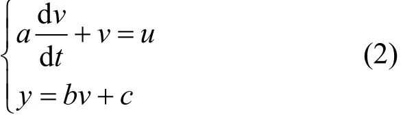
We hope that the expression can represent soft sensor system in all situations, in which the values of parameters may change. Although the expression is linear, it reflects nonlinear characteristics of soft sensor system. We rewrite Eq. (2) in another form for generalization.

In which f(•) represents static model and the parameter of the first part changes or is the same. In some cases, the first part is fixed with some nonlinear model for f(•), and the expression represents Wiener model at this time. Therefore, Eq. (3) can be considered as an extension of Wiener model. Some processes may fit Wiener model [23-25] well, while other cases does not, which will be shown later in case study. When the dynamic characteristics of system change, the static model will compensate to it. Thus, although good estimation results may be provided by Wiener model, its explanation and generalization ability may be limited.

In our opinion, there are more choices for static model of soft sensor systems. When a soft sensor system is around some working point or its nonlinear characteristics is not strong, linear model could be chosen for f(•). Otherwise, nonlinear model is more appropriate [11, 28, 29]. Since chemical process is usually operated under some working condition and soft sensor system is more stable, a linear model is chosen for f(•) in this paper. It is feasible to use Eq. (2) to represent single-input soft sensor system. With linear model, the modeling complexity is reduced and it is easier to use the soft sensor model in applications. Moreover, model parameters have physical meanings. a reflects response time, and b and c are related to static gain and working condition. They can be updated online to track the change of dynamic and static characteristics under different working conditions.

Equation (2) gives a continuous expression of the proposed model for single-input soft sensor system. Its dynamic part builds dynamic relationship between secondary and intermediate variables, which is equivalent to the one between secondary and primary variables with the gain of 1, while the static part builds static relationship between intermediate and primary variables which is equivalent to the one between secondary and primary variables. Therefore, the dynamic relationship between secondary and primary variables can be built depending on not the increments of them but the secondary and intermediate ones. At the same time, the static relationship can be built depending on intermediate and primary variables without the assumption that the system is in steady state.

2.2 Model expression for single-input soft sensor system

Equation (2) has been verified feasible for single-input soft sensor system. In applications, discrete model expression for soft sensor system is preferred. There are many choices for static model and we need some more extensive expression. In this part, we first introduce the discrete expression for Eq. (2), and then an extensive one will be shown. In this paper, we just use Eq. (6) for study.

We have the continuous expression of Eq. (2)

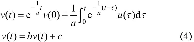
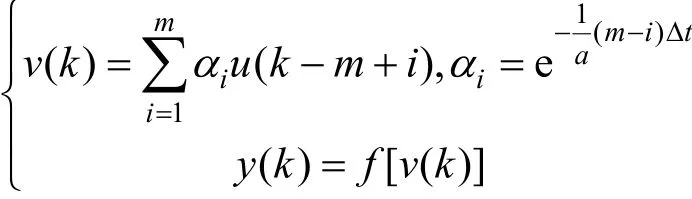
Discreting Eq. (4) and letting v(k)=v(kΔt) and u(k)= u(kΔt), we obtain

The first part of Eq. (6) represents dynamic submodel, with a as parameter, while the second part represents static submodel, with b and c as parameters. The parameters are updated online as working point changes. {,1,2,,} α=… are decay weights. The farther the historical data of secondary variable is from the moment, the smaller the value of the weight is, where

iim

The extensive model expression can be written asin which many model forms can be chosen for f(•), and the parameter of the first part may be fixed or change.

2.3 Model expression for multi-input soft sensor system

In actual processes, a soft sensor system has multiple secondary variables, so the model expression of Eq. (6) is extended to multi-input soft sensor system.

Given the number of secondary variables p, we can use the following transfer function to describe the dynamic relationship between primary and secondary variables [11, 27].

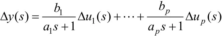
where y represents primary variable and {uj} represents secondary variables. Letting {vj,j=1,2,…,p} be intermediate variables, we use the following equation to describe soft sensor system.

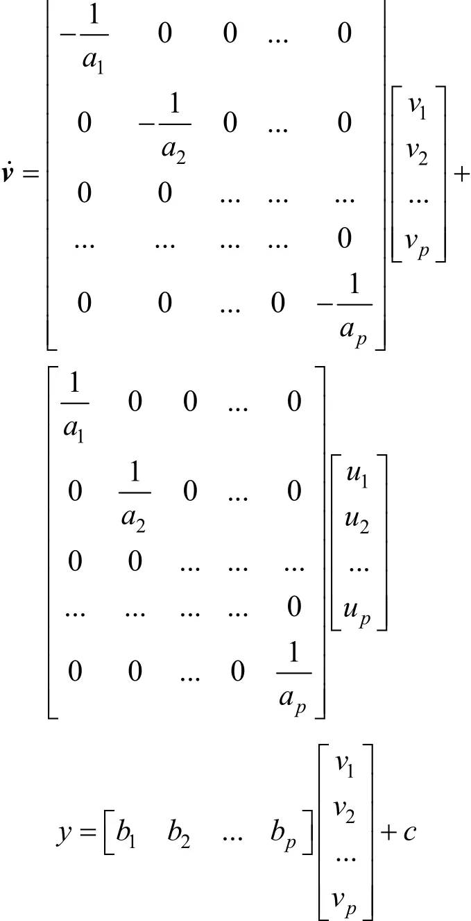
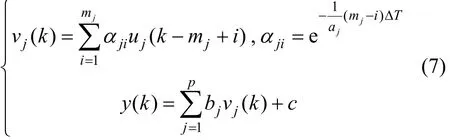
With the same derivation for the model expression of single-input soft sensor system, we have the one for multi-input soft sensor system. =…, and c are the model parameters that may change under different working conditions, related to the response time of system, the gain and working condition change, respectively, {,1,2,,} where the first part of Eq. (7) represents dynamic submodel, the second part represents static submodel. {,1,2,,}=… is the number of historical data of secondary variables. The dynamic relationship between secondary and primary variables is built by the dynamic submodel with secondary and intermediate variables, while the static one is built by the static submodel with intermediate and primary variables.

It should be noted that the values for may be the same or different in theory. Therefore, specific analysis for it is required according to mechanism of soft sensor system, which is helpful for model identification.

2.4 Determination of the number of historical data

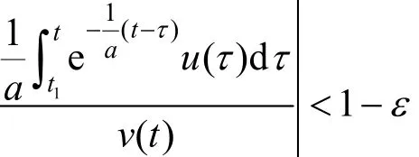
The number of historical data of secondary variable m is an important parameter to determine whether the dynamic submodel fully reflects the dynamic characteristics of the system, thereby affecting the estimation accuracy of the model. Its value corresponds to the integration time interval [t1, t]. With T=t−t1,based on the derivation of m.

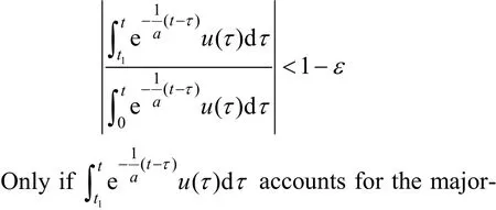
As shown in Eq. (4), for arbitrary sufficiently small positive number ε, t1exists satisfying the following equation. mTt=Δ, where [·] represents the first integer greater than itself. Therefore, m can be obtained through T. The discussion below is for single-input soft sensor system. We can obtain {,1,2,,}

Let λ be the permissible error limit, such as

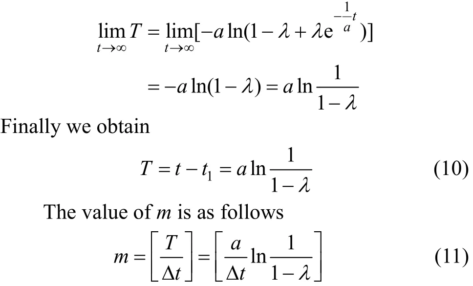
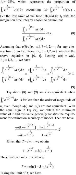
According to Eq. (11), m is related to a and sampling time Δt, which is actually the minimum value ensuring that the dynamic submodel can fully reflect the dynamic characteristics of the system and the estimation accuracy of soft sensor model. Generally, this value is sufficient. Based on Eq. (11), we have {mj, j=1,2,…,p } for a soft sensor system.

{aj} will change at different working points, so the values of {mj} will change accordingly. In applications, {mj} are usually set as some sufficiently large values with less trouble.

3 ALTERNATE IDENTIFICATION ALGORITHM FOR MODEL PARAMETERS

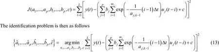
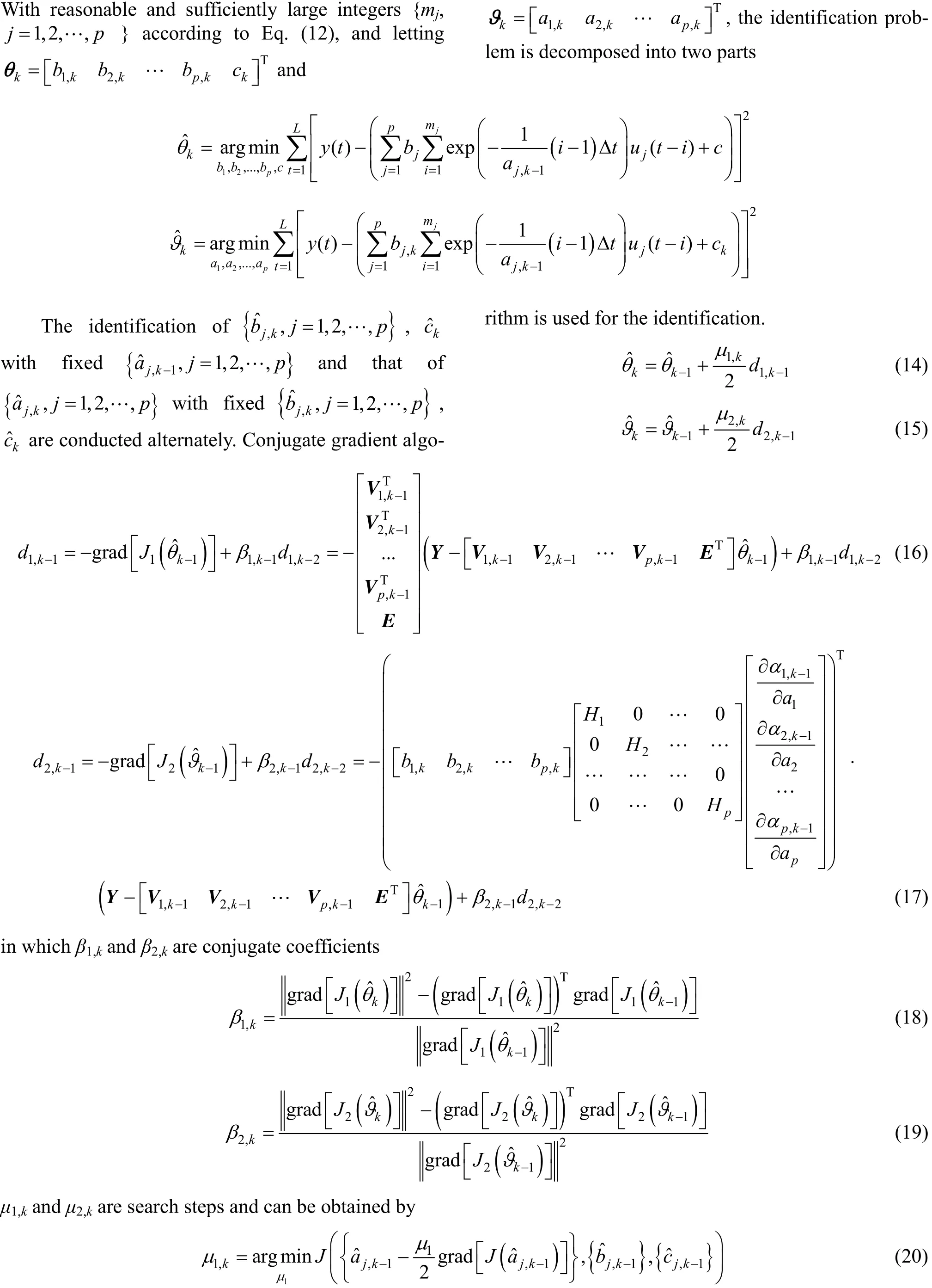
To reduce the difficulty in parameters identification from the model structure [21], we decompose the identification problem into two parts based on the hierarchical principle [22]. The dynamic and static submodels are identified alternately based on the conjugate gradient algorithm. The parameters are updated with the corresponding update method online. The identification algorithm and update method can also be applied to extensive model expression in Section 2.2 and 2.3. Since this paper mainly focuses on modeling for soft sensor system, the choice for the identification algorithm may not be very good. Better algorithm and its improvement will be studied in further work.

With the number of secondary variables p (1,2,p=…), and the number of sample points (u1, u2,…,up,y ) L, the cost function is defined as

4.1 Estimation of pH value

A pH neutralization process in our laboratory is studied as shown in Fig. 2, in which an acid(H2SO4) stream and a base(NaOH) stream that are mixed in a reactor. The acid and base stream flows are secondary variables, and pH value in the reactor is primary variable. We use acid and base stream flows to estimate pH values. It is a multi-rate problem in soft sensor system, since the sample period of primary variables is greater than the secondary variables. However, we mainly study the feasibility and effectiveness of the proposed model, identification algorithm, and update method in single-rate case.

The Wiener model is frequently used to describe the process and the liquid level of reactor is assumed to have smaller fluctuations [30, 31]. From the mechanism of pH neutralization process we know that if liquid level remains unchanged, the process conforms to Wiener model structure completely [32]. However, the change of liquid level should not be neglected in industrial processes, so Wiener model may not describethe dynamic and nonlinear characteristics of pH neutralization process well and the pH values would not be estimated accurately in some cases.

This experiment is conducted for more than 20 min and sampling time is 3 s. The delay time for pH response is about 30 s. We take 300 samples for modeling. The signals for acid and base stream flows are shown in Fig. 3.

To illustrate the effectiveness of the proposed model, support vector machine (SVM) model and Wiener model are used for comparison. SVM model is one of effective static nonlinear models widely used for soft sensor systems. Wiener model consists of autoregressive moving average (ARMA) model in cascade with artificial neural network (ANN) with proper model order and number of neurons. According to the mechanism, the response time for pH value with regard of two secondary variables is the same. We set the initial parameter values of the proposed model a0=400, b10=0, b20=0, and c0=y(0), and y(0) is the initial pH value. The proposed model is identified and updated online based on the identification and update method in Section 3. Fig. 4 shows the estimations for pH values with the proposed model, SVM model and Wiener model. The liquid level of reactor is shown in Fig. 5. It should be noted that we do not have true values for model parameters in the proposed model and there are no tracking curves for these parameters.

Figure 2 The experimental facility

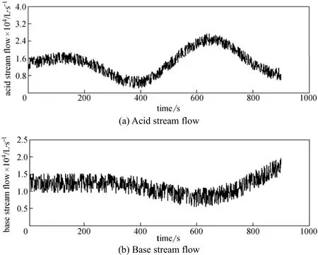
Figure 3 Signals of acid (a) and base (b) stream flows

Figure 4 shows that pH values are estimated more accurately with the proposed model and working condition changes are effectively tracked. The effectiveness of the alternate identification and update method is also reflected. The estimation errors of pH values are larger with SVM model and Wiener model. Compared with static nonlinear model SVM, the proposed model describes the dynamic and static nonlinear characteristics of soft sensor system effectively and provides more accurate estimations for pH values. On the other hand, the fluctuation range of liquid level in Fig. 5 can not be neglected. The Wiener model is not very accurate for pH neutralization process in this study. The parameters of dynamic and static submodels of the proposed model are updated in time to track the change of dynamic and static characteristics.

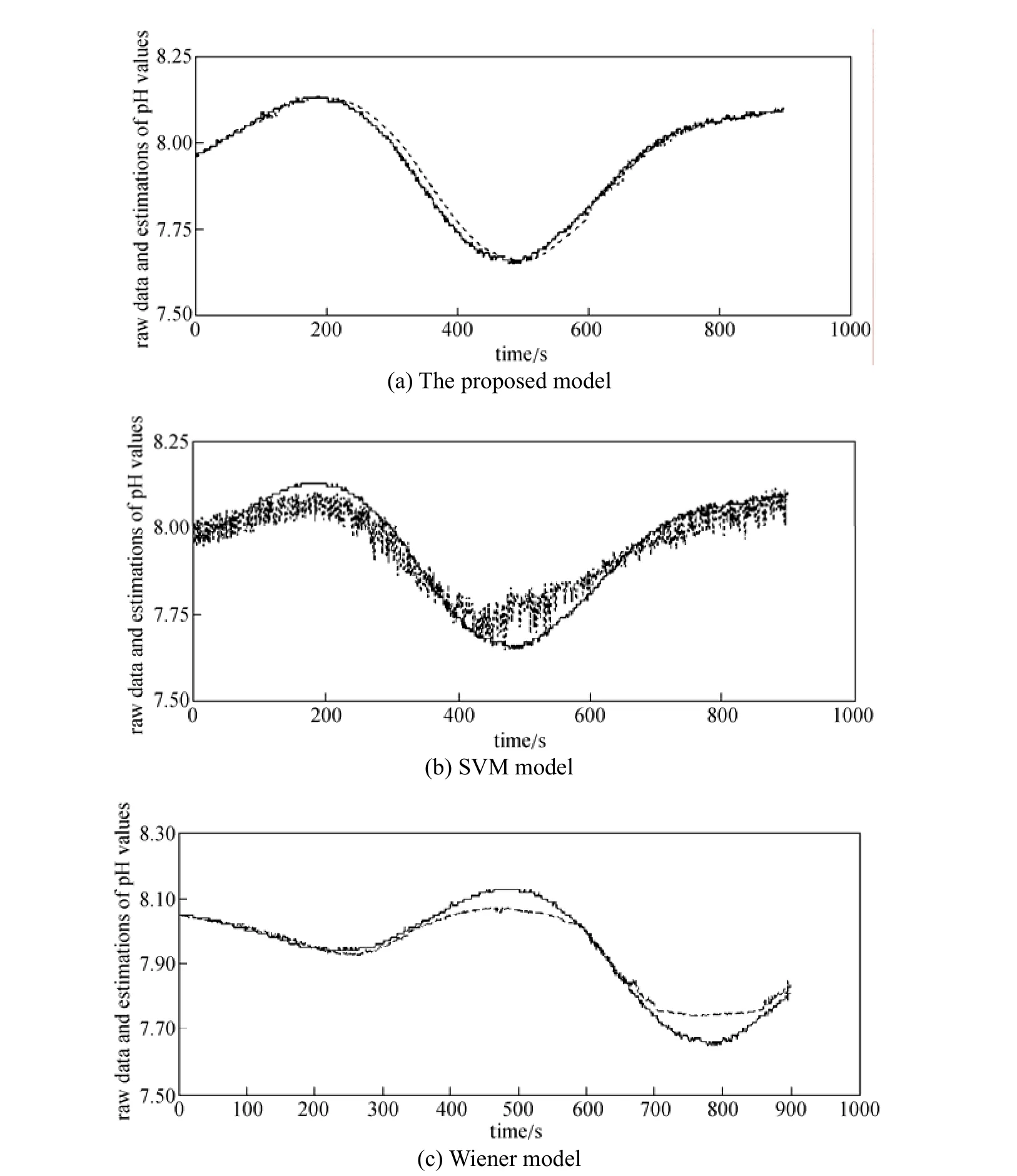
Figure 4 Estimations for pH values based on the proposed model (a), SVM model (b) and Wiener model (c)

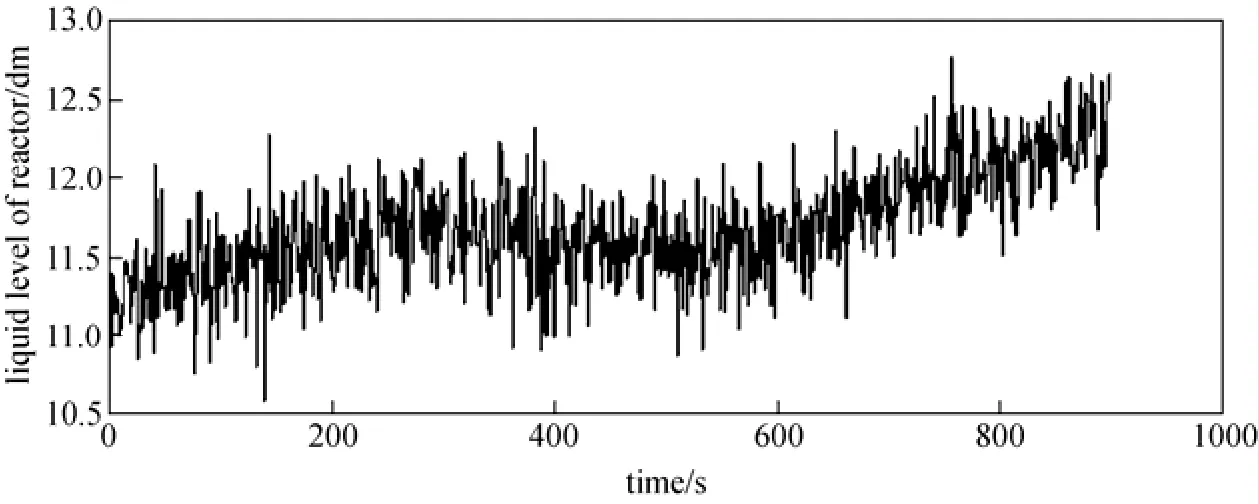
Figure 5 Liquid level in the reactor

Therefore, for this soft sensor system the proposed model is more suitable and effective to estimate pH values.

4.2 Estimation of ethylene concentration

Ethylene distillation tower is important equipmentin ethylene recovery. Its main purpose is to separate high purity ethylene product from hybrid C2 fraction. Generally, ethylene concentration in the product is required to achieve more than 99% and its fluctuation range is required within 0.025%. Ethylene concentration is available from online analytic instrument with more than 20 min delay. It is necessary to establish soft sensor for accurate estimation of ethylene concentration. Two secondary variables are selected according to the mechanism, the pressure at the top of the tower and the temperature on discharge plate.

This simulation experiment of ethylene distillation tower is established based on the dynamic simulation software gPROMS (general process modelling system) and is conducted for 421 min. The sample period for ethylene concentration and all secondary variables is 1 min. The signal of secondary variables is shown in Fig. 6. SVM model and the proposed model are used for estimating ethylene concentration, as shown in Fig. 7. According to the mechanism, there may be different response time for ethylene concentration with regard of two secondary variables. For the proposed model, we set a10=180, a20=180, b10=0, b20=0, and c0=y(0), and y(0) is the initial value for ethylene concentration. The parameters are identified and updated following the algorithms in Section 3. Fig. 7 shows that the difference between the estimation results of two models is not large, but since the control for ethylene concentration is required within 0.025%, the estimation with the proposed model is much better. On the other hand, SVM model is more complex than the proposed model, so the modeling method proposed in this paper is more effective and practical for applications.

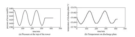
Figure 6 Signals of two secondary variables

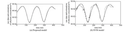
Figure 7 Estimations for ethylene concentration with the proposed model (a), with SVM model (b)

5 CONCLUSIONS

This paper proposes a soft sensor model derived from Wiener model structure which consists of dynamic and static submodels in cascade. The dynamic submodel builds the dynamic relationship between secondary and primary variables, while the static submodel builds their static relationship. These submodels describe the dynamic and static characteristics of soft sensor system separately. The proposed model avoids the integration of processes of building dynamic and static relationships, so the estimation accuracy is improved. This paper also provides an alternate identification algorithm for model parameters. Changes in system characteristics can be tracked based on the update method and the model can describe soft sensor system effectively.

We have just studied the modeling method and identification algorithm in single-rate case. The next step is to improve the modeling method and identification algorithm to achieve multi-rate modeling and parameters update. The alternate identification and update method bring in great calculation, especially when the number of secondary variables is large.Therefore, better identification method and corresponding recursive algorithm are needed.

REFERENCES

1 Kadlec, P., Gabrys, B., Strandt, S., “Data-driven soft sensors in the process industry”, Computers Chem. Eng., 33, 795-814 (2009).

2 Hui, P., Tohru, O., Yukihiro, T., Hideo, S., Kazushi, N., Valerie, H.O., Masafumi, M., “RBF-ARX model-based nonlinear system modeling and predictive control with application to a NOxdecomposition process”, Control Engineering Practice, 12, 191-203 (2004).

3 Dae, S.L., Min, W.L., Seung, H.W., Young, J.K., Jong, M.P.,“Nonlinear dynamic partial least squares modeling of a full-scale biological wastewater treatment plant”, Process Biochemistry, 41, 2050-2057 (2006).

4 Cao, P.F., Luo, X.L., “Modeling of soft sensor for chemical process”, Journal of Chemical Industry and Engineering, 64 (3), 788-800 (2013). (in Chinese)

5 Hector, J.G., Heb, Q.P., Wang, J., “A reduced order soft sensor approach and its application to a continuous digester”, Journal of Process Control, 21, 489-500 (2011).

6 Tian, H.P., David, S.H.W., Jang, S.S., “Development of a novel soft sensor using a local model network with an adaptive subtractive clustering approach”, Industrial & Engineering Chemistry Research, 49 (10), 4738-4747 (2010).

7 Luo, J.X., Shao, H.H., “Developing dynamic soft sensors using multiple neural networks”, Journal of Chemical Industry and Engineering, 54 (12), 1770-1773 (2003). (in Chinese)

8 Elom, D., Huang, B., Xu, F.W., Aris, E., “A decoupled multiple model approach for soft sensors design”, Control Engineering Practice, 19, 126-134 (2011).

9 Hong, B.S., Fan, L.T., John, R.S., “Monitoring the process of curing of epoxy/graphite fiber composites with a recurrent neural network as a soft sensor”, Artificial Intelligence, 11, 293-306 (1998).

10 Dai, X.Z., Wang, W.C., Ding, Y.H., Sun, Z.Y., “Assumed inherent sensor inversion based ANN dynamic soft-sensing method and its application in erythromycin fermentation process”, Computers Chem. Eng., 30, 1203-1225 (2006).

11 Ma, Y., Huang, D.X., Jin, Y.H., “Discuss about dynamic soft-sensing modeling”, Journal of Chemical Industry and Engineering (China), 56 (8), 1516-1519 (2005). (in Chinese)

12 Wu, J.F., He, X.R., Chen, B.Z., “Back-propagation neural network model of dynamic system and its application”, Journal of Chemical Industry and Engineering (China), 51 (3), 378-382 (2000). (in Chinese)

13 Qin, S.J., “Neural networks for intelligent sensors and control-Practical issues and some solutions”, Academic Press, New York (1996).

14 Principe, J.C., Euliano, N.R., Lefebvre, W.C., Neural and Adaptive Systems, Wiley, New York (2000).

15 Eykhoff, P., System Identification—Parameter and State Estimation, John Wiley & Sons, New York (1974).

16 Strejc, V., “Least squares parameter estimation”, Automatica, 16, 535-550 (1980).

17 Juan, C.G., Enrique, B., “Identification of block-oriented nonlinear systems using orthonormal”, Journal of Process Control, 14, 685-697 (2004).

18 Figueroa, J.L., Biagiola, S.I., Agamennoni, O.E., “An approach for identification of uncertain Wiener systems”, Mathmatical and Computer Modelling, 48, 305-315 (2008).

19 Martin, K., Sabina, S., “Identification of Wiener models using optimal local linear models”, Simulation Modelling Practice and Theory, 16, 1055-1066 (2008).

20 Ronald, K.P., Martin, P., “Gray-box identification of block-oriented nonlinear models”, Journal of Process Control, 10, 301-315 (2000).

21 Wang, D.Q., Ding, F., “Least squares based and gradient based iterative identification for Wiener nonlinear systems”, Signal Processing, 91, 1182-1189 (2011).

22 Ding, F., Chen, T.W., “Hierarchical gradient-based identification of multivariable discrete-time systems”, Automatica, 41, 315-325 (2005).

23 Ania, L.C., Osvaldo, E.A., Jose, L.F., “A nonlinear model predictive control system based on Wiener piecewise linear models”, Journal of Process Control, 13, 655-666 (2003).

24 Martin, K., Sabina, S., “Identification of Wiener models using optimal local linear models”, Simulation Modelling Practice and Theory, 16, 1055-1066 (2008).

25 Stefan, T., Hannu, T.T., “Support vector method for identification of Wiener models”, Journal of Process Control, 19, 1174-1181 (2009).

26 Shafiee, G., Arefi, M.M., Jahed-Motlagh, M.R., Jalali, A.A.,“Nonlinear predictive control of a polymerization reactor based on piecewise linear Wiener model”, Chemical Engineering Journal, 143, 282-292 (2008).

27 Fu, Y.F., Su, H.Y., Chu, J., “MIMO soft-sensor model of nutrient for compound fertilizer based on hybrid modeling technique”, Chin. J. Chem. Eng., 15 (4), 554-559 (2007).

28 Shang, C., Gao, X., Yang, F., Huang, D., “Novel Bayesian framework for dynamic soft sensor based on support vector machine with finite impulse response”, IEEE Transaction on Control Systems Technology, DOI: 10.1109/TCST.2013.2278412.

29 Wu, Y., Luo, X.L., Yuan, Z.H., “Soft sensor modeling with dynamic interpolation neutral network for multirate system”, Chemical Industry and Engineering Progress, 28 (8), 1323-1327 (2009). (in Chinese)

30 Gomez, J.G., Jutan, A., Baeyens, E., “Wiener model identification and predictive control of a pH neutralization process”, IEE Proc.—Control Theory Appl., 151 (3), 329-338 (2004).

31 Mahmoodi, S., Poshtan, J., Mohammad, R.J.M., Montazeri, A.,“Nonlinear model predictive control of a pH neutralization process based on Wiener-Laguerre model”, Chemical Engineering Journal, 146, 328-337 (2009).

32 Luo, X.L., Chemical Process Dynamics, Chemical Industry Press, Beijing (2005). (in Chinese)

2013-06-09, accepted 2013-12-21.

* Supported by the National Natural Science Foundation of China (61104218, 21006127), the National Basic Research Program of China (2012CB720500) and the Science Foundation of China University of Petroleum (YJRC-2013-12).

** To whom correspondence should be addressed. E-mail: luoxl@cup.edu.cn