DONG Jie (董杰)

School of Naval Architecture, Ocean and Civil Engineering, Shanghai Jiao Tong University, Shanghai 200240, China, E-mail: qpdongjie@sjtu.edu.cn

WANG Ben-long (王本龙), LIU Hua (刘桦)

School of Naval Architecture, Ocean and Civil Engineering, MOE Key Laboratory of Hydrodynamics, Shanghai Jiao Tong University, Shanghai 200240, China

Run-up of non-breaking double solitary waves with equal wave heights on a plane beach*

DONG Jie (董杰)

School of Naval Architecture, Ocean and Civil Engineering, Shanghai Jiao Tong University, Shanghai 200240, China, E-mail: qpdongjie@sjtu.edu.cn

WANG Ben-long (王本龙), LIU Hua (刘桦)

School of Naval Architecture, Ocean and Civil Engineering, MOE Key Laboratory of Hydrodynamics, Shanghai Jiao Tong University, Shanghai 200240, China

(Received February 7, 2014, Revised September 9, 2014)

The evolution and run-up of double solitary waves on a plane beach were studied numerically using the nonlinear shallow water equations (NSWEs) and the Godunov scheme. The numerical model was validated through comparing the present numerical results with analytical solutions and laboratory measurements available for propagation and run-up of single solitary wave. Two successive solitary waves with equal wave heights and variable separation distance of two crests were used as the incoming wave on the open boundary at the toe of a slope beach. The run-ups of the first wave and the second wave with different separation distances were investigated. It is found that the run-up of the first wave does not change with the separation distance and the run-up of the second wave is affected slightly by the separation distance when the separation distance is gradually shortening. The ratio of the maximum run-up of the second wave to one of the first wave is related to the separation distance as well as wave height and slope. The run-ups of double solitary waves were compared with the linearly superposed results of two individual solitary-wave run-ups. The comparison reveals that linear superposition gives reasonable prediction when the separation distance is large, but it may overestimate the actual run-up when two waves are close.

run-up, double solitary waves, nonlinear shallow water equations (NSWEs)

Introduction

Recently, a few giant tsunami events caused severe damage on the near-shore region in different countries. It is related to a classic research topic of long wave run-up on a plane beach in tsunami studies. Tsunami waves usually appear as a wave train when they attacked coastlines. Studies of the run-up of multiple waves could give insight into the dynamic behaviors of tsunami waves and inundation on coasts. Moreover, the run-up process of multiple waves also brings about sediment transport and wave-structure interactions, so it is useful to assess the influence of tsunami in coastal region.

The nonlinear shallow water equations (NSWEs) are commonly used to study the propagation and runup of long waves for the cases that the nonlinearity of waves is more important than the dispersion. For a simple flow domain, e.g., a plane beach, analytical solution of run-up of long waves can be found. Carrier and Greenspan proposed the hodograph transformation to solve NSWEs with a moving shoreline which transfers NSWEs into a second-order linear differential equation, and gave an analytical solution of the boundary value problem for the NSWEs[1]. Based on the Carrier and Greenspan’s transformation, Antuono and Brocchini[2]provided an approximate solution of the boundary value problem by using a perturbation approach solely using the assumption of small amplitude waves. Synolakis[3]found different run-up regi-mes for the run-up of breaking and non-breaking solitary waves through the asymptotic solutions and a series of laboratory experiments. With the NSWEs, Li and Raichlen[4]proposed an analytic solution of runup of a nonbreaking solitary wave on plane beaches and concluded that the maximum run-up predicted by the nonlinear model is larger than that obtained by Synolakis[3]and other linear solutions available. The fully nonlinear and highly dispersive Boussinesq equations were used by Zhao et al.[5]to investigate the evolution and run-up of solitary waves and N-waves on plane beaches. They discussed variations of the potential energy and the kinematic energy during the run-up and rundown on a plane beach. Further, Zhao et al.[6]carried out numerical simulation of tsunami waves propagating on the continental shelf with an extremely gentle slope. It is interesting to note that, from the numerical results obtained by the Boussinesq model, the N-shape tsunami waves could evolve into long wave trains, undular bores or solitons near the coastal area for the cases of different initial wave heights. Through numerical simulations of run-up of a solitary wave on a plane beach using the Boussinesq equations and the shallow water equations respectively, Liang et al.[7]reported that the maximum run-up of a solitary wave predicted by the Boussinesq model is identical with that practiced by the shallow water model even though there is a significant difference of the surface elevation during the propagation and runup of a solitary wave on a plane beach. Chan and Liu[8]developed a Lagrangian numerical model to solve the nonlinear shallow water equations and investigated the evolution and run-up of non-breaking long waves on a plane beach. It was found that for a single wave the accelerating phase of the incident wave controls the maximum run-up height.

Although single solitary wave run-up has been extensively studied, little literature on the run-up process of double solitary waves is available, which can have important application on estimating the run-up of waves with multiple crests and have been observed during tsunami events[9,10]. El et al.[11]showed by theory that a sequence of isolated leading solitons forms as an undular bore propagates into decreasing water depth. Viotti et al.[12]discussed conditions for extreme wave run-up on vertical barrier and indicated that the runup of long strongly nonlinear waves trains impinging on a vertical wall can exceed six times the far-field amplitude of the incoming waves. Recently, laboratory studies of the run-up of double solitary waves with equal wave amplitudes or unequal wave amplitudes on steep slopes were carried out by Xuan et al.[13]. More cases of the double solitary waves of equal wave amplitudes were considered in the laboratory experiments by Lo et al.[14]. They also reported the flow field of double solitary waves during the process of run-up on a plane beach measured with particle image velocimetry. The intensity of the backwash flow generated by the first wave strongly is considered to affect the run-up height of the second wave.

In the present study, a numerical model based on NSWEs is applied to simulate the process of long waves on a beach. The model is validated by the runup of a solitary wave and double solitary waves using analytical solutions[2]and laboratory data[3,4,13,14]. The process of double solitary waves on a plane beach is obtained. The characteristics of the first wave run-up and the second wave run-up are summarized in different separation distances. The ratios of the second maximum run-up to the first one are supposed to be related to the unified separation factor. The present numerical solutions are compared with the linear superposed results of two individual solitary waves.

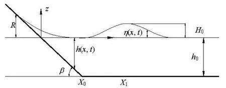
Fig.1 Definition sketch of run-up of long waves

1. Mathematic formulation and numerical method

1.1Mathematic formulation

We consider the run-up of two-dimensional long wave incident upon a uniform sloping beach as shown in Fig.1. The classical NSWEs are

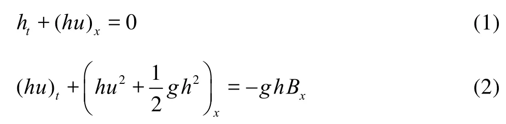
in whichhis the total water depth,uthe depth-averaged horizontal velocity of fluid flows with the free surface,gthe gravitational acceleration andBthe bottom surface elevation relative to the still water surface level.His the wave height,η(x,t) =h(x,t)+B(x) is the wave profile,X0is the position of toe,X1is the position of wave crest,βis the angle of beach andRis the run-up.B(x) =-h0is the still water depth atx＞X0.

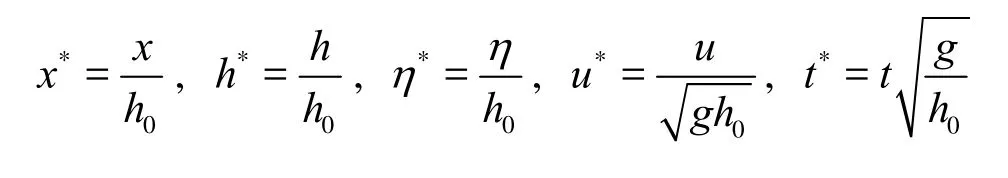
For convenience, leth0be the characteristic length and introduce the following non-dimensional variables:The relative wave heightH/h0is simplified toεand slope tanβis replaced ofsin the remaining discussion.

These equations belong to a general class of hyperbolic system

Equation (3) is similar to the Euler equations in gas dynamics in mathematical structure, which can admit discontinuous solutions even though the boundary values are continuous. Hence, it is a key procedure to employ an appropriate numerical scheme to solve them.

1.2Numerical method

We adopted the finite volume method (FVM), not considering the source term on the right side of Eq.(3)

whereF~inis the second-order correction term. More details about the numerical algorithm can be found in Ref.[15].

1.3Boundary conditions

When NSWEs are applied to simulate wave problems, it is difficult to deal with the open boundary and the moving shoreline boundary. To efficiently impose different boundary conditions, “ghost cells” were added to the outmost grids. We updated cells adjacent to boundaries using ghost cells values. For the open boundary at which the incident waves should be described, the wave profile and velocity were known before the computation:

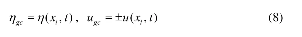
whereηgcandugcare the values on ghost cells,0ηandu0are the given surface elevation and velocity of incident waves. We used two rows of ghost cells here. For the free outflow boundary and the wall boundary, the values on ghost cells were extrapolated from cells in domain

whereηanduare the computed surface elevation and velocity. The positive one in Eq.(8) represents the the free outflow boundary and the negative one stands for the wall boundary. For the Godunov-type method used here, the numerical flux at each interface is split into two directions. The flux are consisted by two parts,A+ΔQi=1andA-ΔQi=1in Eq.(5). Namely, the reflected wave would propagate out freely withA-ΔQi=1and incoming waves are generated into the domain withA+ΔQi=1. Therefore, the open boundary serves as a non-reflecting boundary. Suppose that a monochromatic wave is generated at the left of a wave flume with a flat bottom and reflected by a vertical wall at the right end. The incident wave elevation and velocity areHere, the length of wave flume with a flat bottom is 100 m and still water depthh0=1m. Snapshots of the surface elevation of steady standing wave along the wave flume are shown in Fig.2. It is found that the numerical algorithm works well for the open boundary working as a wave generation boundary without the second reflection of the reflected waves propagating from the computational domain.

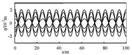
Fig.2 Snapshots of suface elevation of standing waves along wave flume

Moreover, the moving shoreline need to solve the Riemann problems with an initial dry state on one side. A threshold, called dry tolerance, is used to distinguish wet or dry. The numerical flux in Eq.(6) is given by the mathematical solutions of the Riemann problem with a dry state. This treatment is a common technique used in the run-up simulations, see Refs.[16,17]. We will not discuss it in detail here.

2. Numerical model setup and validation

2.1Wave breaking and dispersive term

There are two different run-up regimes of nonbreaking and breaking waves. Synolakis[3]proposed the following breaking criterion for solitary waves

The dispersive term is neglected in NSWEs. As a consequence, wave front will be steeper until breaking. To avoid the deformation of wave in propagation, waves are generated right at the toe of slope. The nonreflecting open boundary ensures that the reflected wave back from slope propagates outward freely. Moreover, wave amplitudes are relatively small on account of non-breaking conditions. Therefore, for nonbreaking long waves on a slope, the dispersion is not significant to the nonlinearity.

2.2Single solitary wave

We utilized the first-order solution of the KdV equations to give the wave profile and velocity at the open boundary:

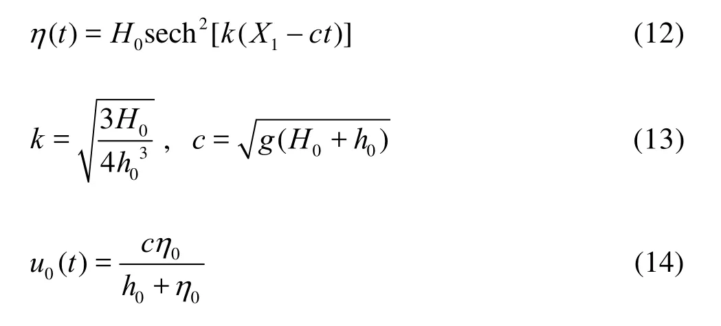
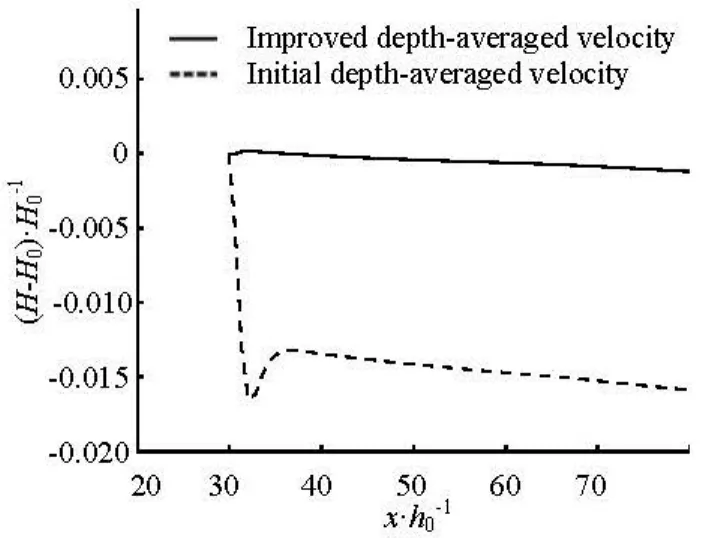
Fig.3 Solitary wave height damping along the flume withH 0=0.1m andh0=1m

whereX1is the initial phase,cthe wave phase velocity, andu0(t) the depth-averaged horizontal fluid velocity. In the numerical practices, we improved the steady of solitary-wave shape by implying more precise depth-averaged velocity. When Eq.(14) was used to generate a solitary wave, there would be a trailing wave after a few of time steps, which leads a decrease of the target wave height. The reason is that the velocity of water particles is not accurately equal to wave phase celerityc. Due to the hypothesis of verticallyaveraged velocity in shallow water equations, it is very similar to the physical wave paddle in laboratory. Hence, following the experience of Xuan et al.[13], we used the improved Goring wave generation methodology:

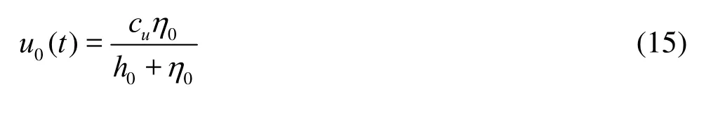
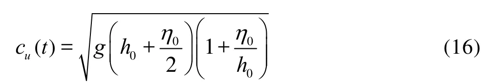
The unsteady phase velocitycu(t) changes with the water level instead the original constant phase velocityc. The results of wave height damping along the flume using these two different values of wave celerity are shown in Fig.3. It is indicated that the modified celerity can help to improve the velocity field and maintain initial wave heights.

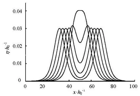
Fig.4 Wave profiles of double solitary waves forε=0.03 andσfrom 1.3 to 0.3 with an interval 0.2

2.3Double solitary waves

A dimensionless parameterσis defined as the ratio of the distance between two crests of two solitary waves to the effective wavelength of single solitary waveL. Here, the effective wavelengthLof a solitary wave is defined by

wheret0is the initial time of computation. Figure 4 shows the wave profile of double solitary waves with equal wave heights and various separation distances. Whenσis equal to 0.3, the two waves merge into one single-peak wave. Whenσequals to 0.5, wave weights of the double solitary waves are not identical with the wave height of elementary solitary waveH0. For instance, wave height is 0.0316h0instead of 0.03h0withε=0.03 double solitary waves. Therefore, the minimum value ofσherein is 0.35.

Fig.5 Shoreline time series of solitary-wave run-up withε= 0.0185 on a 1:19.85 slope

2.4Numerical parameters and model validation

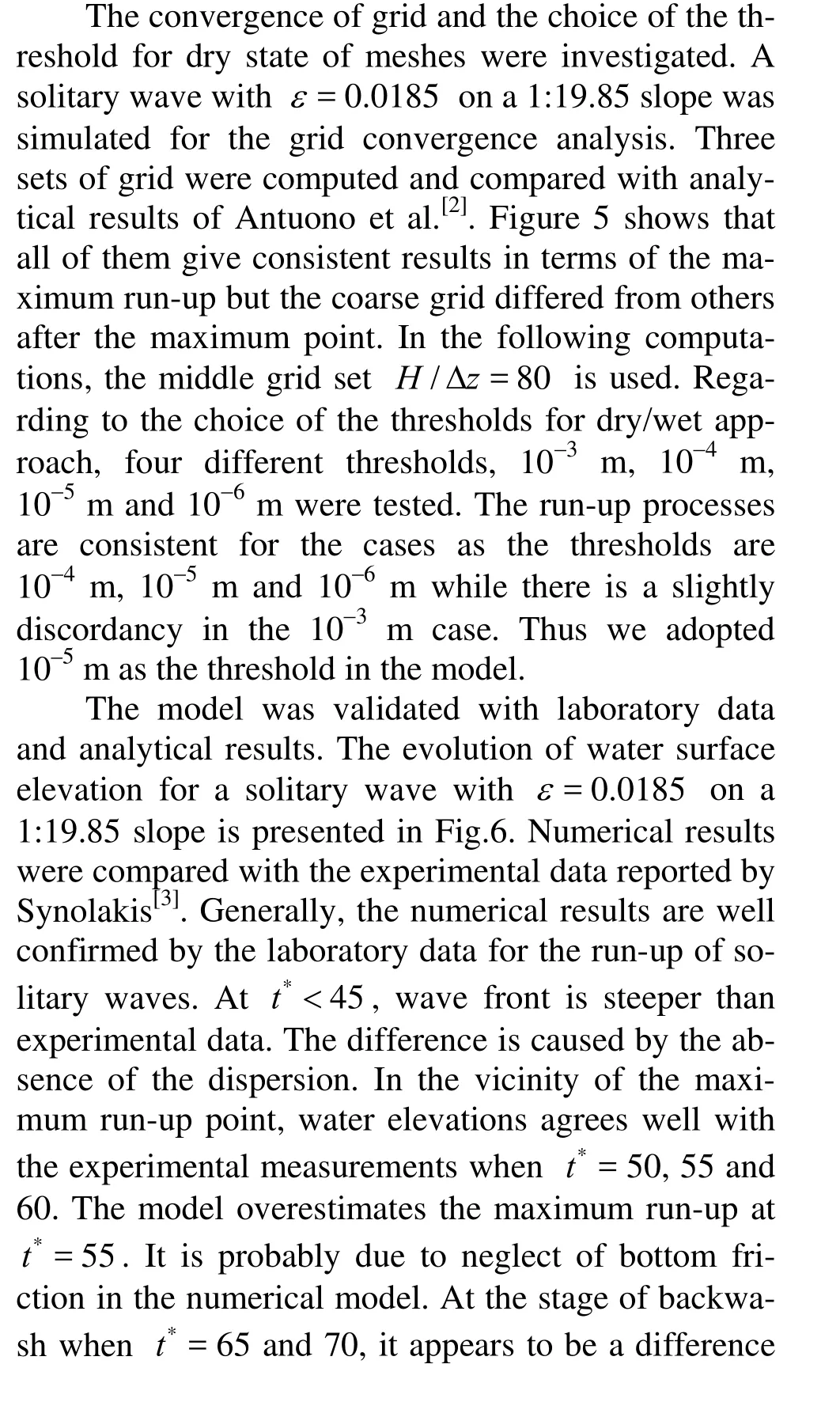
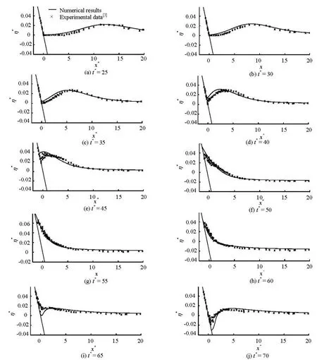
Fig.6 Evolutions of a solitary wave with ε= 0.0185 on 1:19.85 slope

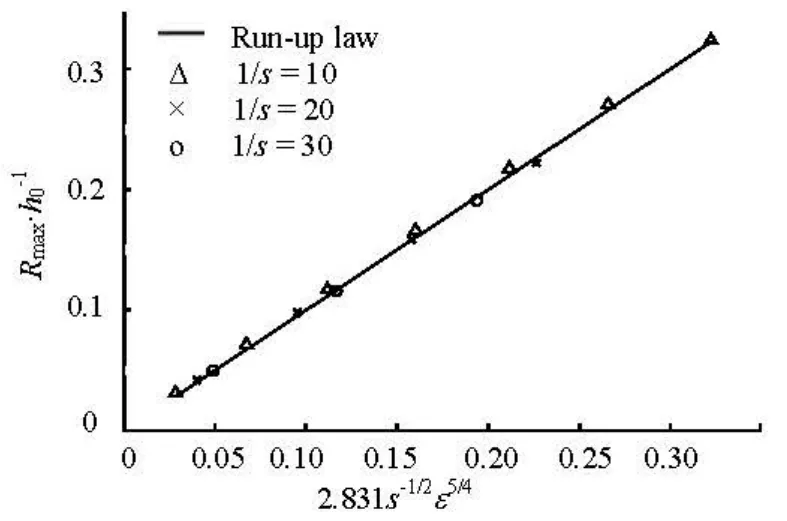
Fig.7 Comparison of numerical results and the run-up law

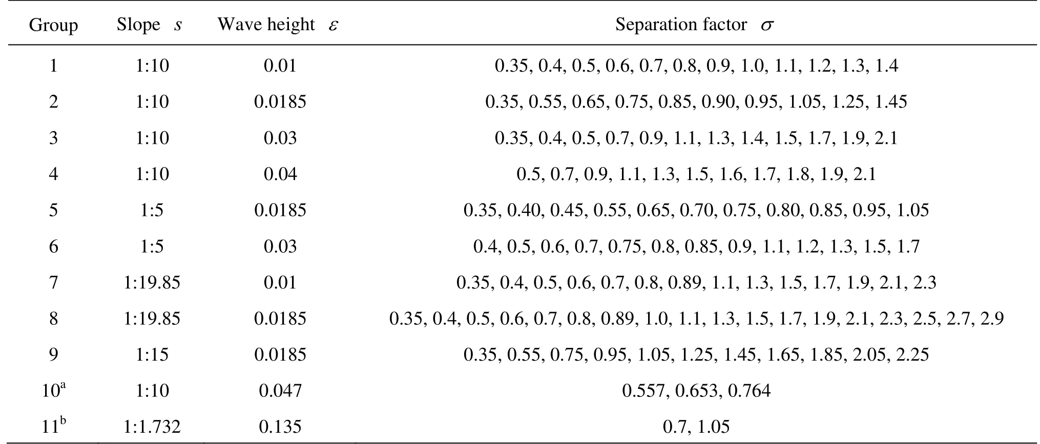
Table 1 Numerical wave conditions of double solitary waves

whereRmaxis the maximum run-up. Figure 7 shows that the maximum run-up of solitary waves agrees well with the run-up law. The numerical model is valid for run-up of non-breaking solitary waves.

3. Results and discussion

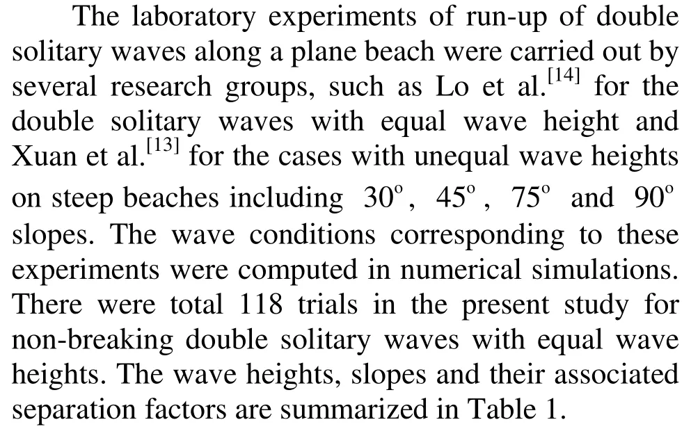
Fig.8 Shoreline time series of solitary-wave run-up with differentεands

3.1Characteristics of run-up of single solitary wave

Due to double solitary waves consisting of two successive solitary waves, the run-ups of double solitary waves are related to run-up of single solitary wave. Let us revisit the characteristics of run-up of single solitary wave. Equation (21) indicates that runup of single nonbreaking solitary wave depends on the beach slope and the wave height. The run-ups of solitary waves with different values ofεandsare shown in Fig.8. When the wave height or the slope is changed, the minimum rundown and duration of overall process will be consequently altered as well as the maximum run-up. For non-breaking solitary waves, Synolakis[3]derived an approximate expression for run-up height in terms of an integral involving the Bessel functions. According to the analytic solution of run-up, the time when the wave reaches its maximum run-up can be defined by

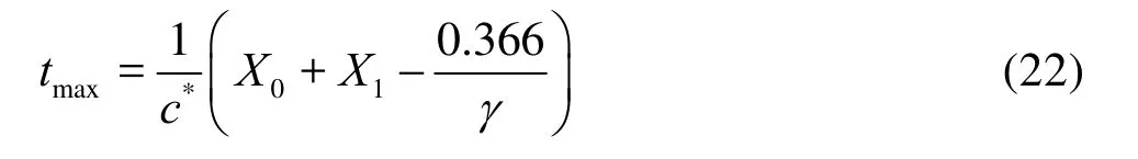
wherec*is non-dimensional celerity and letc*=1. As is shown in Fig.1,X0andX1are non-dimensional length. The non-dimensional wave numberγisγ=(0.75ε)0.5. With Eq.(22), the time when a solitary wave climbed up to the maximum height can be accurately predicted. We find thattmaxfor different values ofεon a slope withs=1:19.85is nearly at the same time, buttmaxis supposed to be significantly changed on different slopes. We set 5% as the limit of error. Namely, when (0.366/γ)/(X0+X1) ＜ 5%, the time of maximum run-up is mainly related to slope excluding wave height. The error limit can be simplified inanother form

Fig.9 Evolutions of double solitary waves with ε =0.0185 and σ =0.35 on 1:19.85 slope

Considering the condition (ε)1/2s-1＞＞ 0.288, it reveals that whenε1/2s-1＞ 4.23, the timetmaxat the maximum run-up is mainly affected by the slope. Whenε1/2s-1＜ 4.23,tmaxis related to not only slope but also wave height. Unfortunately, the timetminwhen minimum rundown appears is not available in analytical solutions. From Fig.8, it is interesting to note thattminis influenced by both slope and wave height. The characteristic duration ΔTof run-up is herein defined by (tmax-tmin). With qualitative observation from Fig.8, the duration ΔTis longer when the slope is milder or the wave height is smaller. Elsewise, the milder slope or larger wave height would cause the sharp trough curve at minimum rundown, which is probably because of nonlinearity.

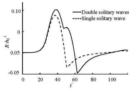
Fig.10 Shoreline movement of 0.0185 double solitary waves on a 1:19.85 slope

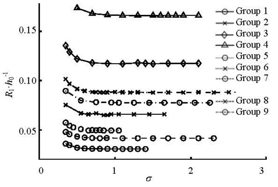
Fig.11 The first run-up heights of double solitary waves with differentσ. The annotation of symbols are consistent in Fig.12 and Fig.13

3.2Free surface profiles and shoreline movement of double solitary waves

Fig.12 The second run-up height of double solitary waves with different values ofσ

Fig.13 The ratio of the second run-up height to the first one of double solitary waves with different values ofσ

Fig.14 Unified run-up ratio of double solitary waves with normalizedσ*

The free surface profiles for an incident double solitary waves with the wave heightε=0.0185 and separation factorσ=0.35 are presented in Fig.9 for different non-dimensional times. The results of double solitary waves can be compared with wave profiles of single solitary wave in the corresponding times. Waves are non-breaking in both run-up and backwash process. The two wave crests are too close to figure out in Figs.9(a)-9(c). The water elevations in the rear face of the first wave are lifted in contrast to the case of single solitary wave. Double solitary waves climbup the slope with more water body and the corresponding maximum run-up is higher than that of single solitary wave. After the time when maximum run-up appears, water body began to back wash offshore. However, due to the presence of the incoming second wave, water body near the shoreline is pushed to inshore again leading to the second run-up as shown in Fig.9(i). For single solitary wave, the minimum rundown appears in Fig.9(j) while the water elevation starts to set down for the case of double solitary waves. From Fig.9(l), we find that the minimum rundown of double solitary waves is lower than that of single solitary wave and the timetminis also smaller than that of single solitary wave. As a result, the duration of the whole process is longer than that of single solitary wave.

Table 2 Comparison of presnet computation and experimental measurment

The time series of shoreline movement with nondimensional time is shown in Fig.10. The shoreline movement of double solitary waves withε=0.0185 on a slope with 1/s=19.85 is compared with results of single solitary wave. There are two peaks in the time series of shoreline movement, which stand for the first run-up and the second run-up. The second maximum run-up is remarkably lower than the first one for this case.

3.3Maximum run-ups of double solitary waves

The maximum run-up of the first wave and the second wave of double solitary waves are plotted in Figs.11 and 12, respectively, with respect to separation factorσ. In general, the maximum run-ups of the first wave do not change withσexecpt a few cases thatσis a little more than 0.35. The silghtly incrases of the first maximum run-up is because the incidient wave peak heights are increased when two wave creasts are too close, which has been discussed previously. From Fig.12 it can be seen that the second maximum run-ups are significantly varied with the seperation factorσ. When the seperation factor gradually decrease, i.e., when two waves are located nearer initially, the second maximum run-ups firstly slightly increase and afterwards decrease rapidly. It could be conluded that the second run-up process is strongly affected by the first wave.

Since the first run-up almost does not change, we unified the run-ups of double solitary waves with the ratio of the second maximum run-up to the first maximum run-up,R2/R1. From Fig.13 it can be seen that the ratioR2/R1is fluctuating in the vicinity of 1 withσ=0.35-3. The attenuation is remarkable whenσis small. The highest points whenR2/R1reaches its maximum are not consistent. The tendencies of attenuation with different wave conditions are also not the same. Hence, we normalized the separation factorσwith the relative wave heights and slopes, and the final unified results are plotted in Fig.14. With the normalized transformation, the values of ratioR2/R1are identical with respect to seperation factorσ. A unified seperation factorσ*is defined as

As is shown in Fig.14, whenσ*is greater than 0.6, corresponding to point A, the ratioR2/R1approximately equals 1, i.e., the second run-up of double solitary waves is not influenced by the first one. Whenσ*is located in the range from 0.27 to 0.6, i.e., from point C to point A, there is a slight amplification of the second wave run-up. The amplification is about 5%. It is remarkable and difficult to be measured in laboratory experiments. No experimental data reported the amplification probably because of experimental error. Behind point C, when*σminishes from 0.27 to 0, the second maximum run-ups are significantly influenced by the first wave. The minimum values appeares, whenσ*=0, in range of 0.58 to 0.78. This range of the minimum ratio of run-ups is due to the wave heights of double solitary waves and the slope of plane beach.

With the unified seperation factor, numerical results of group 10 and group 11 in Table 1 are compared with experimental data as shown in Table 2. Note that the distance between double solitary waves creasts are defined by diffirent methods in the experiments.

Fig.15 Comparison of double solitary waves run-up and linearly superposed run-up with ε =0.0185 and s=1:19.85

These separation distance between two crests in space are transformed to the present seperation factorσin time as in Eq.(20). The deviations between present computation and laboratory data are evaluated by

The numerical model has overpredicted the attenuation of the second wave run-up within 12%. The comparisons are not enough for the following reasons. Firstly, the first run-ups of the numerical model are not consistent with experimental results, whose reasons were explianed in Lo et al.[14]. Apart from the discordance of run-up measurement, waves in group 10 trend to break according to Eq.(11) withξb=0.5139. On the other hand, with the unified separation factorσ*, we find that wave conditions of group 10 locate at range ofσ*=0 to 0.27 in Fig.14 and the unified factorσ*of group 11 are far greater than 0.6, which means that the distance of two wave crests is too far to interact with each other during the run-up process. Finally, the double solitary wave shape would change in a wave flume when the two waves are close enough initially. The incidient wave heights of double solitary waves are actually not equal which were disscussed in Ref.[13]. Details of the disagreement of numerical results and laboratory data need to be investigated futher.

3.4Linear superposition of two individual wave runups

To understand wave-wave interaction of two successive solitary waves approaching a plane beach, it is interesting to compare the numerical results of runup of double solitary waves and the linearly superpo-sed results of two run-ups of single solitary wave with a time delay. The delay could be calculated byσL/cin Eq.(20). The comparisons of different separation factorσwith aε=0.0185solitary wave on a 1:19.85 slope are shown in Fig.15. Figures 15(a) and 15(b) suggest that the linearly superposed run-up results overestimate the run-up of double solitary waves. When the separation factor increases from 0.7 to 2.1, the run-up time series of double solitary waves is consistent with ones linearly superposed. The difference is probably because the wave-wave interaction are strong when the two waves are too close. As was mentioned above, when wave heights are large or slopes are mild, nonlinearity in rundown process becomes significant where the curve of shoreline time series at minimum rundown becomes a sharp trough. The interaction at this region is difficult to predict using linear superposition of two individual run-up results.

4. Concluding remark

A numerical model based on shallow water equations including the moving shoreline boundary, has been developed for the run-up of long waves. The model has been validated by analytical solutions and experimental data. The non-breaking run-up of double solitary waves on a plane beach is simulated. With the numerical results, it reveals that run-up of the first wave of double solitary waves is not changed with the separation factor. Run-up of the second wave is strongly influenced by the first wave when the separation factor gradually decreases. The tendency is firstly a slight amplification about 5% and a rapid attenuation when two waves are closing. A unified separation factor related to wave heights and slopes has been proposed. With the unified factor, it is found that 0＜σ*＜ 0.27 is the attenuation zone, 0.27 ＜σ*＜ 0.6 is the amplification zone andσ*＞0.6 is the undisturbed zone. Finally, the linear superposition of two individual solitary-wave run-ups are compared to run-ups of double solitary waves. It turns out that the run-ups of double solitary waves can be modeled by the linear superposition of run-ups of two individual solitary waves with a time delay except the case where two waves are close enough.

[1] CARRIER G. F., WU T. T. and YEH H. Tsunami runup and draw-down on a plane beach[J]. Journal Fluid Mechanics, 2003, 475: 79-99.

[2] ANTUONO M., BROCCHINI M. The boundary value problem for the nonlinear shallow water equations[J]. Studies in Applied Mathematics, 2007, 119(1): 73-93. [3] SYNOLAKIS C. E. The run-up of solitary waves[J]. Journal Fluid Mechanics, 1987, 185: 523-545.

[4] LI Y., RAICHLEN F. Solitary wave run-up on plane slopes[J]. Journal of Waterway Port Coastal Ocean Engineering, 2001, 127(1): 33–44.

[5] ZHAO X., WANG B., LIU H. Characteristics of tsunami motion and energy budget during run-up and rundown processes over a plane beach[J]. Physics of Fluids, 2012, 24(6): 062107.

[6] ZHAO X., LIU H. and WANG B. Evolvement of tsunami waves on the continental shelves with gentle slope in the China Seas[J]. Theoretical and Applied Mechanics Letters, 2013, 3(3): 032005.

[7] LIANG D., LIU H. and TANG H. et al. Comparison between Boussinesq and shallow-water models in predicting solitary wave run-up on plane beaches[J]. Coastal Engineering Journal, 2013,55(4): 1350014.

[8] CHAN I.-C., LIU P. L-F. On the run-up of long waves on a plane beach[J]. Journal of Geophysical Research, 2012, 117(C8): C08006.

[9] GRUE J., PELINOVSKY E. N. and FRUCTUS D. et al. Formation of undular bores and solitary waves in the Strait of Malacca caused by the 26 December 2004 Indian Ocean tsunami[J]. Journal of Geophysical Research, 2008, 113(C5): C05008.

[10] MADSEN P. A., FUHRMAN D. R. and SCHAFFER H. A. On the solitary wave paradigm for tsunamis[J]. Journal of Geophysical Research, 2008, 113(C12): C12012.

[11] EL G. A., GRIMSHAW R. H. J. and TIONG W. K. Transformation of a shoaling undular bore[J]. Journal of Fluid Mechanics, 2012, 709: 371-395.

[12] VIOTTI C., CARBONE F. and DIAS F. Conditions for extreme wave runup on a vertical barrier by nonlinear dispersion[J]. Journal of Fluid Mechanics, 2014, 748: 768-788.

[13] XUAN Ruan-tao, WU Wei and LIU Hua. An experimental study on run-up of two solitary waves on plane beaches[J]. Journal of Hydrodynamics, 2013, 25(2): 317-320.

[14] LO H. Y., PARK Y. S. and LIU P. L-F. On the run-up and back-wash processes of single and double solitary waves–An experimental study[J]. Coastal Engineering, 2013, 80: 1-14.

[15] LEVEQUE R. J. Finite volume methods for hyperbolic problems[M]. Cambridge, UK: Cambridge University Press, 2002, 311-348.

[16] GEORGE D. L. Augmented Riemann solvers for the shallow water equations over variable topography with steady states and inundation[J]. Journal of Computational Physics, 2008, 227(6): 3089-3133.

[17] GEORGE D. L. Adaptive finite volume methods with well-balanced Riemann solvers for modeling floods in rugged terrain: Application to the Malpasset dam-break flood (France, 1959)[J]. International Journal for Numerical Methods in Fluids, 2011, 66(8): 1000-1018.

[18] MADSEN P. A., SCHÄFFER H. Analytical solutions for tsunami runup on a plane each: single waves, N-waves and transient waves[J]. Journal of Fluid Mechanics, 2010, 645: 27-57.

10.1016/S1001-6058(14)60103-7

* Project supported by the National Natural Science Foundation of China (Grant No. 51379123), the Natural Science Foundation of Shanghai Municipality (Grant No. 11ZR1418200) and the Shanghai Water Authority and the State Key Laboratory of Ocean Engineering, Shanghai Jiao Tong University (Grant No. GKZD010063).

Biography: DONG Jie (1988-), Male, Ph. D. Candidate

LIU Hua, E-mail: hliu@sjtu.edu.cn