LIU Hou-lin (刘厚林), LIU Dong-xi (刘东喜), WANG Yong (王勇), WU Xian-fang (吴贤芳),

WANG Jian (王健), DU Hui (杜辉)

Research Center of Fluid Machinery Engineering and Technology, Jiangsu University, zhengjiang 212013, China, E-mail: liuhoulin@ujs.edu.cn

Experimental investigation and numerical analysis of unsteady attached sheetcavitating flows in a centrifugal pump*

LIU Hou-lin (刘厚林), LIU Dong-xi (刘东喜), WANG Yong (王勇), WU Xian-fang (吴贤芳),

WANG Jian (王健), DU Hui (杜辉)

Research Center of Fluid Machinery Engineering and Technology, Jiangsu University, zhengjiang 212013, China, E-mail: liuhoulin@ujs.edu.cn

(Received July 1, 2012, Revised March 20, 2013)

This paper studies the attached sheet cavitation in centrifugal pumps. A pump casted from Perspex is used as the test subject. The cavitation bubbles were observed in the entrance of the impeller and the drops of the head coefficients were measured under different operating conditions. A Filter-Based Model (FBM), derived from the RNG k-εmodel, and a modified Zwart model are adopted in the numerical predictions of the unsteady cavitating flows in the pump. The simulations are carried out and the results are compared with experimental results for 3 different flow coefficients, from 0.077 to 0.114. Under four operating conditions, qualitative comparisons are made between experimental and numerical cavitation patterns, as visualized by a high-speed camera and described as isosurfaces of the vapour volume fractionαv=0.1. It is shown that the simulation can truly represent the development of the attached sheet cavitation in the impeller. At the same time, the curves for the drops of the head coefficients obtained from experiments and calculations are also quantitatively compared, which shows that the decline of the head coefficients at every flow coefficient is correctly captured, and the prediction accuracy is high. In addition, the detailed analysis is made on the vapour volume fraction contours on the plane of span is 0.5 and the loading distributions around the blade section at the midspan. It is shown that the FBM model and the modified Zwart model are effective for the numerical simulation of the cavitating flow in centrifugal pumps. The analysis results can also be used as the basis for the further research of the attached sheet cavitation and the improvement of centrifugal pumps.

centrifugal pump, attached sheet cavitation, high-speed camera, modified Zwart model, Filter-Based Mode (FBM)

Introduction

In liquid flows, if the pressure drops to a point below the saturated vapour pressure, the liquid will change its thermodynamic state by forming vapourfilled cavities. This phenomenon is generally associated with undesired effects and is known as the cavitation. There are several types of cavitation in the hydro-machinery, and a very common form is the sheet cavitation, which is defined as a closed vapour region attached on the impeller blades. The cavitation can cause a significant reduction in performance, as manifested by the reduced mass flow rates in the pumps, the load asymmetry, the noise, the vibration and the erosion. In addition, it is found that the cavitation erosion is mainly related with the length of the sheet cavity, as well as the circumferential speed and the properties of the impeller material. To avoid or minimize the harms caused by the sheet cavitation, it is desirable to study the occurrence, the extent and the behavior of the sheet cavitation in the initial design stages.

The CFD plays an important role in the flow field analysis, the advanced commercial CFD software can be used for a wide range of flows, including the cavitating flows[1,2]. Over the last decade, due to the advancement of the physical modelling and the computational capabilities for cavitating problems, the methods based on the Navier-Stokes equations in computing cavitating flows have received increasinglymore attention. Generally speaking, these methods are divided into the following three main categories: the interface tracking method[3], the barotropic equation models[4,5], and the Transport equation models (TEM)[6,7]. Among them, the TEM is the most widely used strategy, where the flow is treated as a two-phase system with mass transfer between the vapour and liquid phases. In these models, either the simplified Rayleigh-Plesset (R-P) equation[6], or the empirical formula[7]are used to establish the interphase mass transfer rates. In particular, the Zwart model is implemented in several general purpose CFD solvers, and is successfully used to solve problems in various engineering applications. However, due to the significant effect of the turbulence on the cavitating flows, before the Zwart model is applied to the numerical simulation of the present study, an improvement is made to the Zwart model by modify the formula of the phasechange threshold pressure following the idea of Singhal et al..

It is important to note that most of cavitating flows are in the state of turbulence. So the choice of the turbulence model in the numerical predictions of the cavitating flows is very important. To simulate the cavitating turbulent flows, various approaches were developed, and the Reynolds-Averaged Navier-Stokes (RANS) equations are widely used to deal with the turbulence[8]. The RANS equations, with eddy viscosity models, such as the standard k-εand RNG k-εmodels, are widely used in the numerical predictions of various cavitating flows, to obtain acceptable predictions with presently available computational resources. However, Okabayashi et al. pointed out that the RANS approach is model-dependent, consequently, it is not very useful to deal with the interactions between the cavitation and the turbulence. Besides, for unsteady cavitating flows, with the RANS method, the large-scale unsteady characteristics can not be adequately identified in the cavitating flows. Recently, the Large Eddy Simulation (LES) approach, initially proposed by Smagorinsky and modified by many researchers, has become a tool for unsteady turbulent cavitating flows[9]. In the approach, the space-averaging or the filtering is used, which could quite accurately predict the turbulent transient information in a wide range of applications. Sato et al. studied the vortex cavitation in a double-suction volute pump, they found that with the LES, more detailed vortex structures can be captured, furthermore, by using a high-order turbulent LES model, it is possible to capture the vortex cavitations brought about by the turbulence at the upstream side of an impeller. However, there are some limitations of the LES method. This method requires a very fine grid within the boundary layer to simulate a large number of small-scale fluctuations in the boundary layer, involving a large computing resource, which restricts the application of the LES for the complicated turbulent cavitating flows in the rotating machinery.

In order to make up the deficiencies of the two methods, Johansen et al.[10]formulated a Filter-Based Model (FBM), which combines the standardk-ε model with the large eddy simulation. In recent years, the FBM is gradually applied to the simulation of turbulent cavitating flows. Wu et al.[11], Tseng and Shyy[12], Huang and Wang[13], Wei et al.[14]compared the methods of RANS and FBM in the application of the cavitating flows around the hydrofoil. They found that the FBM can not only help reduce the indeterminacy associated with the conventional eddy viscosity models and the turbulent quantities at the inlet by decreasing the dependence on the eddy viscosity, but also are the velocity distributions and the unsteady cavity shapes obtained by the FBM more consistent with experimental visualizations than the results obtained with the RANS. In addition, Wang et al.[15]evaluated the predictive capability of several turbulence models for the performance of an axial-flow pump. They found that FBM can accurately predict the output characteristics of the axial flow pump at the design point, and compared to other three eddy viscosity models, the FBM can significantly improve the prediction accuracy at the off-design points.

In the present study, the experimental investigation focuses on the cavitation performance curves and the development of the attached sheet cavitation in the entrance of the impeller, and a high-speed camera is used to observe the cavitation bubbles. In the numerical prediction, the modified Zwart model and the filter-based model are added to the CFX through the second development technology, and the simulations are carried out with three different flow coefficients, from 0.077 to 0.114. Under four operating conditions, qualitative comparisons are made between experimental and numerical cavitation patterns. At the same time, the cavitation performance curves obtained from experiments and calculations are also quantitatively compared. In addition, a detailed analysis is performed on the vapour volume fraction contours on the plane of span is 0.5 and the loading distributions around the blade section at the midspan.

Fig.1 Sketch of the closed experiment rig

1. Experiments

1.1 Experiment facility

The experimental facility for cavitations in the Jiangsu University is a closed and recirculating waterflow loop consisting of a vacuum pump, a reservoir tank, four butterfly valves, a turbine flowmeter, a regulating tank, two sphericalvalves and the test section. A sketch of the experiment rig is shown in Fig.1. The facility water is held in the 4.5 m3stainless steel reservoir tank. The water leaves the tank and then enters the 0.09 m diameter stainless steel piping system. The test section located in the middle of the facility system is the essential component of the experiment facility.

1.2 Image acquisition system

The development of cavitation bubbles is observed traditionally from the side of the pump. This, of course, involves only a part of bubbles in the impeller passage. In the present study, to better observe the cavitation bubbles in the entrance of the impeller, a water tank casted from Perspex is attached to the pump. The water inlet is placed at the side of the water tank to facilitate the working of the high-speed camera, and a vent is set on the roof of the tank to release the gas in the tank. In addition, considering that the attached tank should have little influence on the pump performance and play a role in stabilizing the flow, the volume of the tank is designed as 0.1 m3. A photograph of the water tank is shown in Fig.2.

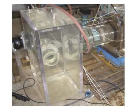
Fig.2 The photograph of the water tank

The images of the cavitation bubbles in the entrance of the impeller are taken with the high-speed camera of Y-series4L with a spatial resolution of 1 024×1 024 pixels. Its maximum shooting rates are 4 000 frames/s and 256 000 frames/s at the full resolution and the non-full resolution, respectively. The pixel size is 14 µm×14 µm and the memory is 16G, the continuous shooting time is about 45 s at the full resolution. The illumination is provided by a LED lamp and two halogen lamps, the LED lamp has no effect on the temperature of the fluid as it is a cold light source. The power of the halogen lamp is 750 W. The light of the LED lamp from the side of the volute goes into the pump during the shooting, and two halogen lamps are placed at both sides of the inlet tube. In the present experiment, the shooting rate of the highspeed camera is set to 3 000 frames/s, so that the impeller rotates about 3ofor each shot. Figure 3 shows the relative position of the experimental equipment (test section).

Fig.3 The layout of the experimental equipment

Fig.4 The photograph of the test pump

Table 1 Important parameters of the pump

Fig.5 Front view of the impeller and names of various parts

1.3 Test pump

The test pump used in the present study is a centrifugal pump with a five blade impeller, a diffuser and a volute. The pump is also casted from transparent Perspex, and made into a square structure in the out-side but a circular one in the inside to reduce the refraction of light, as shown in Fig.4.

The geometry parameters of the centrifugal pump for experiment and simulation are given in Table 1.

Figure 5 shows the front view of the impeller and the names of various parts, used in the analysis of experimental and simulated results.

2. Mathematical model

2.1 Governing equations

The governing mixture equations for mass and momentum are

The liquid-vapour mass transfer due to the cavitation is modelled by a vapour volume fraction transport equation

where uiis the velocity vector,ρmis the mixture density,pvis the vapour density,ρlis the liquid density, αvis the vapour volume fraction,µand µtare the mixture dynamic viscosity and the turbulent viscosity, respectively,Reand Rcare the mass transfer source terms related with the evaporation and the condensation of the liquid and vapour phases in the cavitation.

The mixture densityρmand the mixture dynamic viscosityµare defined as

2.2 Modified Zwart model

According to theR-P equation, the size variations of a single vapour bubble are governed by the pressure difference between the phase-change threshold pressure and the local static pressure. Neglecting the second-order terms and the surface tension force, the R-P equation is simplified to

This equation provides a physical method to incorporate the influence of the bubble dynamics into the cavitation model. Assuming that all vapour bubbles in a system share the same size, Zwart et al. proposed that the total interphase mass transfer rate(R)is related with the number of bubbles per unit volume (n0)and the mass transfer rate of a single bubble as

The expression of n0depends on the direction of the phase change. For the bubble growth (evaporation),n0is given by

For the bubble collapse process (condensation), n0is given by

Equations (5)-(8) can be combined to derive the source terms in Eq.(3) for the evaporation and condensation as

Further, to incorporate the significant effect of the turbulence on the cavitating flows into the Zwart model, a Probability Density Function (PDF) method is used for considering the effect of the turbulent pressure fluctuation (Pturb), and the phase-change threshold pressure is modified via the PDF method. This method requires the estimation of the values ofPturb, is found to be simple and robust and would yield better results.

where pvis the phase-change threshold pressure,psatis the saturated vapour pressure,αnucis the nucleation site volume fraction,RBis the radius of a nucleation site,Fvapand Fcondare empirical parameters regulating the rate of evaporation and condensation, respectively. In the CFX, the coefficients mentioned above are set as follows:αnuc=5.0×10–4,RB=1.0×10–6, Fvap=50,Fcond=0.01. Due to the fact that the evaporation is usually much faster than the condensation, the value ofFvapis larger than that of Fcond.

2.3 Filter-based model

In the Johansen’s approach, the expression and the constants ofkandεequations are unchanged, however, the formula for the turbulent viscosity µtis derived by a filtering procedure

where Cµ=0.09,Fis the filter function defined in terms of the ratio of the filter sizeΔand the turbulent length scale

After adding the filter functionF, when the turbulence size is smaller than the filter size, the RNG k-εmodel will be recovered, on the other hand, the formula for the turbulent viscosityµtis changed into the following form

Then, this model has a consistent form to the one equation LES models.

It is important to note that to ensure the filter process, in the present study, the filter size is chosen to be no less than the largest grid scale adopted in the calculation, namely,Δ≥ max(Δ x Δ y Δ z)1/3,Δx,Δyand Δzare the lengths of the grid in the three coordinate directions, respectively.

3. Computational methodology

The calculation domain includes 5 sub-domains: the impeller, the diffuser, the volute, the prolongations for impeller inlet and the volute outlet, which is to reduce the influence of the large velocity gradient on the computation results. All simulations are performed on the hexahedral mesh generated by ICEM-CFD. In order to reduce the influence of the grid number on the computation results, a grid dependency study at the design point under the non-cavitation condition is carried out firstly, namely, the steady calculations are carried out with different grid numbers. It is found that the head correlation is less than 1% and there is almost no difference among the pressure fields around the leading edge.Consequently, the influence of the grid numbers on the numerical results can be ignored. Finally, all the simulation results presented hereafter are obtained with a mesh of 1.66×106cells, as shown in Fig.6.

Fig.6 the structured mesh of the computational domain

The numerical simulations are performed by using the commercial CFD code ANSYS-CFX 12, based on the Control Volume-Based Finite Element Method (CV-FEM). The linearized equations of momentum and continuity are solved simultaneously with an Algebraic Multigrid method based on the Additive Correction Multigrid strategy. The implementation of this strategy in the ANSYS-CFX is very robust and efficient in predicting the swirl flows in the turbomachinery.

Under the cavitation or non-cavitation conditions, the settings of the boundary conditions are specifiednearly the same.Generally speaking, on the inlet boundary, the total pressure is imposed and on the outlet boundary, the mass flow rate is set. As to the wall boundary condition, no slip condition is enforced on the wall surface. In the cavitating cases, the volume fraction of the vapour and the water are assumed to be 0 and 1, respectively.

First, a steady state calculation for each case is performed, and then an unsteady state calculation is performed with the steady calculation result as the initial condition. Define the time for the impeller to rotate 360oas one calculation periodT . According to the rotation speed n=1 450 r/min, the period can be obtained,T =0.041 s and set ΔT=0.000345 s. Therefore, there are 120 time steps during a calculation period, with the impeller rotating 3oper time step. The total time of the unsteady calculation is6T , and the cavitation characteristics at the last period are analyzed.

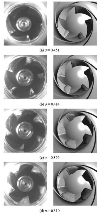
Fig.7 Qualitative comparison among the cavitation bubbles observed in the leading edge of the blades

4. Analyses of results

For the convenience of dealing with the results from experiments and calculations, the data will be transformed with the help of three dimensionless numbers, namely, the flow coefficientφ, the head coefficientψand the cavitation number σ, defined as

where Pinis the static pressure at the pump inlet,H is the pump head,u2is the outlet peripheral speed.

4.1 Cavitation bubbles

Figure 7 shows a qualitative comparison among the patterns of the attached sheet cavitation obtained by experiments and simulations, under four different operating conditions, i.e., (φ=0.096,σ=0.451), (φ=0.096,σ=0.414), (φ=0.096,σ=0.376), (φ= 0.096,σ=0.31). The experimental cavitation bubbles are captured by the high-speed camera, the simulated ones are predicted using the FBM turbulence model in combination with the modified Zwart cavitation model and depicted as isosurfaces of αv=0.1[17]. From Fig.7, it is seen that the simulation results are slightly overestimated as compared with the experiment ones.

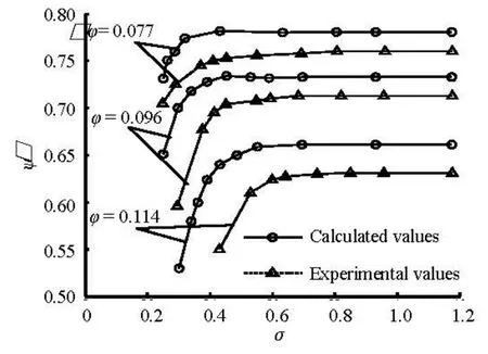
Fig.8 Comparisons between calculated results and experimental results

4.2 Cavitation performance curves

Figure 8 shows the experimental and computed results under different operating conditions. The cavitation is made to occur by gradually reducing the cavitation number, the initial decrease of the cavitation number has no effect on the energy characteristics of the pump, and the head coefficients remain unchanged, when the value ofσcontinues to decrease, the intensity of the cavitaiton is gradually increased, resulting in the decrease of the head coefficient.

According to Fig.8, the simulation results are close to the experimental values for each flow coefficient. It is interesting to note that not only the cavitation patterns are overestimated, but also the predicted head coefficientψare higher than the experimental ones. This result can be explained by the following two reasons: first, the gap between the impeller shroud and the pump cover is not considered in the numerical simulation, in addition, the volume loss and the sudden expansion loss in the impeller outlet, etc. are also not considered, thus the simulated head coefficients would be slightly higher than the experiment values, second, all cavitation models, including the Zwart model and the Full Cavitation Model (FCM), are based on a series of simplifications and assumptions, and the corrections of the model coefficients are based on the test results of the hydrofoil, therefore, there are still significant deficiencies need to be further improved when the cavitation models are applied to the simulation of the cavitating flows in the rotating machinery. In the existing researches, the simulated cavitation size obtained by other scholars are often larger than the experimental values[18,19]. In conclusion, although there are slightly differences between the simulated and the experimental results, we can still say that the simulation can truly describe the development of the attached sheet cavitation in the impeller and the drop of the pump performance.

We can also observe an interesting phenomenon in the process of dealing with the predicted results. When the value of σdecreases, the global performance (head coefficientψ) of the pump slightly rises up, which also can be observed in Fig.8, e.g., (φ=0.077, σ=0.432), (φ=0.096,σ=0.451), (φ=0.114,σ= 0.553). This phenomenon may be associated with an incidence effect: due to the blockage effect of the cavitation, the meridional flow velocity decreases and subsequently contributes to a local increase of the effective angle of attack. However, this phenomenon has not been observed in our experiment.

Table 2 The critical cavitation numbers obtained by calculations and experiments

In order to quantitatively compare the results obtained by experiments and simulations, the critical cavitation number is used, which is defined as the cavitation number corresponding to the reduction of 3 percent of the head coefficient. The predicted and experimental critical cavitation numbers are listed for three different flow coefficients in Table 2.

As shown in Table 2, the comparison demonstrates that the simulation accuracy is high. The gap between the predicted and experimental critical cavitation numbers could be attributed to the following reasons: the shortcomings of the CFD software and the possible errors in the casting of the test pump. Therefore, the FBM turbulence model and the modified Zwart model are effective for the numerical simulation of the cavitating flow in centrifugal pumps.

Fig.9 Vapour volume fraction distribution on the plane of span is 0.5, blade-to-blade view

4.3 Vapour volume fraction distribution on the plane of span is 0.5

To further study the influence of the development of the cavitation on the pump performance, the contours of the vapour volume fraction distribution on the plane of span is 0.5 at the design point is shown in Fig.9 and the span defines the dimensionless distance (between 0 and 1) from the hub to the shroud.

For σ=0.451, the thin attached sheet cavities can be clearly seen on the suction side, attaching to the leading edge of the impeller blades, when the value ofσdecreases, the length of the sheet cavities grows substantially. For σ=0.376, a cavity generates on the pressure side of the blade leading edge, for σ=0.31 the cavity almost interacts with the cavity at the trailing edge of the neighboring blade, at this time, the channel is remarkably obstructed by the cavities, generating a large blockage to the internal flow, which directly contributes to the break-down of the performance of the pump. Obviously, the distribution of cavities in the impeller passage is asymmetrical. The presence of the volute, which not only breaks the axial symmetry of the pump, but also has coupling effects with the impeller, which makes the pressure distribution on the blade surface asymmetrical.

4.4 Blade loading distributions at midspan

Three blades are selected to analyze the influenceof the cavitation on the loading distributions. Figure 9 shows the loading distributions around the blade section at the midspan for different values of σat φ= 0.096. The loading is defined as the pressure difference between the static pressures on the pressure side and the suction side. The locations of blades in the pump are shown in Fig.6. In Fig.10, the streamwise (S)location is the dimensionless distance from the inlet to the outlet of the impeller, ranging from 0 to 1.

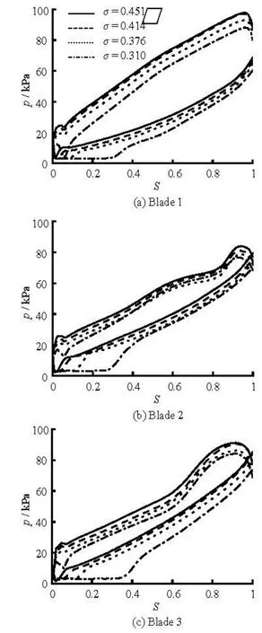
Fig.10 Impeller blade loading distributions at midspan,φ= 0.096

As can be seen from Fig.10, the loading variation on blade 2 is similar to that on blade 3, and is significantly different from that on blade 1. The loading on blade 1 increases from the leading edge to the neighborhood of the trailing edge, while the loadings on blades 2 and 3 have much less changes, which probably due to the fact that blade 1 is much closer to the tongue than other blades, so the volute may affect the loading distributions significantly and the rotor-stator value ofσdecreases to 0.31, the pressure at the leading edge on the suction side almost keeps constant, the blade loading increases fromS =0.05 to S=0.4, but the development of the cavitation has no influence on the loading distribution at the location fromS= 0.4 to S=1, which indicates that the development of interaction here is clearly seen. In addition, the pressure variation on the pressure side is more complex than that on the suction side and the pressure on the pressure side sees a remarkable reduction both at the leading edge and the trailing edge, on the other hand, the pressure on the suction side consistently grows from the leading edge to the trailing edge, and reaches its maximum at the exit.

The initial decrease of the cavitation number almost has no effect on the blade loading. When the the cavitation has a significant influence on the blade loading at the leading edge, and the loading increase is mainly due to the change of the suction side pressure distribution near the leading edge; on the blade near the tongue, the loading is the largest.

5. Conclusions

The experimental investigation and the numerical prediction of the attached sheet-cavitating flows in a centrifugal pump are presented in this paper. A brief summary of the major findings is as follows.

In experimental study, by adding the water tank, the development of the attached sheet cavitation in the whole entrance of the pump can be clearly observed. Thin sheet cavities can be seen on the suction side, attaching to the leading edge of the impeller blades, when the value ofσdecreases, the length of the sheet cavities grows substantially. The development of the cavitation also causes the drop of the pump performance, namely, the reduction of the head coefficients.

In the unsteady numerical prediction, with due considerations of the shortcomings of RANS and LES, a filter is proposed in the simulation of the attached sheet-cavitating flows in centrifugal pumps. The simulation results, including the cavitation patterns and the cavitation performance drop curves are analyzed and compared to the experimental values. In addition, a detailed analysis is performed on the vapour volume fraction contours on the plane of span is 0.5 and the loading distributions around the blade section at the midspan.

Finally, the experiment results are in a good agreement with the numerical simulation results, which indicates that the development of the attached sheet cavitation and the drop of performance in the centrifugal pump can be precisely evaluated by the experimental techniques and the computational methodology implemented in this study, thus providing a good guidance for the initial design of the pumps. Furthermore, the results of this study can also be used asthe basis for the further research of attached sheet cavitation in pumps.

[1] LIU Hou-liu, REN Yun and WANG Kai et al. Research of inner floe in a double blades pump based on OPENFOAM[J]. Journal of Hydrodynamics, 2012, 24(2): 226-234.

[2] LIU Hou-liu, WANG Yong and YUAN Shou-qi et al. Effects of blade number on characteristics of centrifugal pumps[J]. Chinese Journal of Mechanical Engineering, 2010, 23(6): 742-747.

[3] LIU Li-jun, LI Jun and FENG Zhen-ping. A numerical method for simulation of attached cavitation flows[J]. International Journal for Numerical Methods in Fluids, 2006, 52(6): 639-658.

[4] COUTIER-DELGOSHA O., FORTES-PATELLA R. and REBOUD J. L. et al. Stability of preconditioned Navier-Stokes equations associated with a cavitation model[J]. Computers and Fluids, 2005, 34(3): 319-349.

[5] ESFAHANIAN V., AKBARZADEH P. and HEJRANFAR K. An improved progressive preconditioning method for steady non-cavitating and sheet-cavitating fl ows[J]. International Journal for Numerical Methods in Fluids, 2010, 68(2): 210-232.

[6] SINGHAL A. K., ATHAVALE M. M and LI H. et al. Mathematical basis and validation of the full cavitation model[J]. Journal of Fluids Engineering, 2002, 124(3): 617-624.

[7] KUNZ R. F., BOGER D. A. and STINEBRING D. R. et al. A preconditioned Navier-Stokes method for twophase flows with application to cavitation prediction[J]. Computers and Fluids, 2000, 29(8): 849-875.

[8] DING H., VISSER F. C. and JIANG Y. et al. Demonstration and validation of a 3D CFD simulation tool predicting pump performance and cavitation for industrial applications[J]. Journal of Fluids Engineering, 2011, 133(1): 1-14.

[9] LU N.-X., BENSOW R. E. and BARK G. LES of unsteady cavitation on the delft twisted foil[J]. Journal of Hydrodynamics, 2010, 22(5Suppl.): 784-791.

[10] JOHANSEN S. T., WU J. Y. and SHYY W. Filter-based unsteady RANS computations[J].International Jour- nal of Heat and Fluid Flow, 2004, 25(1): 10-21.

[11] WU J. Y., WANG G. Y. and SHYY W. Time-dependent turbulent cavitating flow computations with interfacial transport and filter based models[J]. International Journal for Numerical Methods for Fluids, 2005, 49(7): 739-761.

[12] TSENG Chien-Chou, SHYY W. Modeling for isothermal and cryogenic cavitation[J].International Journal of Heat and Mass Transfer, 2010, 53(13): 513-525.

[13] HUANG Biao, WANG Guo-yu. Evaluation of a filterbased model for computations of cavitating flows[J]. Chinese Physics Letters, 2011, 28(2): 1-4.

[14] WEI Ying-Jie, TSENG Chien-Chou and WANG Guo-Yu. Turbulence and cavitation models for time-dependent turbulent cavitating flows[J]. Acta Mechanicha Sinica, 2011, 27(4): 473-487.

[15] WANG Guo-yu, HUO Yi and ZHANG Bo et al. Evaluation of turbulence models for predicting the performance of an axial-flow pump[J]. Transactions of Beijing Institute of Technology, 2009, 29(4): 309-313(in Chinese).

[16] ZHOU Ling-jiu, WANG Zheng-wei. Numerical simulation of cavitation around a hydrofoil and evaluation of a RNG k-εmodel[J]. Journal of Fluids Engineering, 2008, 130(1): 1-7.

[17] MEDVITZ R. B., KUNZ R. F. and BOGER D. A. et al. Performance analysis of cavitating flow in centrifugal pumps using multiphase CFD[J]. Journal of Fluids Engineering, 2002, 124(2): 377-383.

[18] BONAIUTI D., ZANGENEH M. and AARTOJARVI R. et al. Parametric design of a waterjet pump by means of inverse design, CFD calculations and experimental analyses[J]. Journal of Fluids Engineering, 2010, 132(3): 1-15.

[19] POUFFARY B., FORTES-PATELLA R. and REBOUD J. L. et al. Numerical simulation of 3D cavitating flows: Analysis of cavitation head drop in turbomachinery[J]. Journal of Fluids Engineering, 2008, 130(1): 1-7.

10.1016/S1001-6058(11)60375-3

* Project supported by the National Natural Science Funds for Distinguished Young Scholar (Grant No. 50825902), the Natural Science Foundation of Jiangsu Province (Grant Nos. 51239005, 51179075).

Biography: LIU Hou-lin (1971), Male, Ph. D., Professor