LUO ZHONG-XUAN,FENG ER-BAOAND HU WEN-YU

(1.School of Mathematical Sciences,Dalian University of Technology,

Dalian,Liaoning,116024)

(2.School of Software,Dalian University of Technology,Dalian, Liaoning,116620)

Computing Numerical Singular Points of Plane Algebraic Curves∗

LUO ZHONG-XUAN1,2,FENG ER-BAO1AND HU WEN-YU1

(1.School of Mathematical Sciences,Dalian University of Technology,

Dalian,Liaoning,116024)

(2.School of Software,Dalian University of Technology,Dalian, Liaoning,116620)

Given an irreducible plane algebraic curve of degree d≥3,we compute its numerical singular points,determine their multiplicities,and count the number of distinct tangents at each to decide whether the singular points are ordinary.The numerical procedures rely on computing numerical solutions of polynomial systems by homotopy continuation method and a reliable method that calculates multiple roots of the univariate polynomials accurately using standard machine precision.It is completely different from the traditional symbolic computation and provides singular points and their related properties of some plane algebraic curves that the symbolic software Maple cannot work out.Without using multiprecision arithmetic,extensive numerical experiments show that our numerical procedures are accurate,efficient and robust,even if the coefficients of plane algebraic curves are inexact.

numerical singular point,multiplicity,ordinary,homotopy continuation

1 Introduction

Singular points and their related properties play an important role in the theory of plane algebraic curves(see[1–2]),such as the computation of the genus of an algebraic curve. Practically,singular points present some shape features,such as nodes,self-intersections or cusps of real curves arising from computer aided geometry design,robot motion planning and machine vision.And computing singular points helps to determine the geometric shape and topology of the real curves.

Some of the existing research in CAGD on computing singular points considers rational parametric curves.The computation of singular points of a rational parametric curve is studied in[3].Chenet al.[3]surveyed other methods brie fl y therein.

Singular points of the plane algebraic curve f(x,y)=0 can be computed by solving the polynomial system

where fx(x,y)and fy(x,y)are the partial derivatives of f(x,y)with respect to x and y respectively.Most of the existing methods in[4–8]solved this polynomial system either by resultant computation,which required the exact input of coefficients of algebraic curves,or by the Grbner basis method described in[9].For singular points of high multiplicity or algebraic curves with complex structures,the resultants may become difficult to compute. Furthermore,coefficients of algebraic curves obtained by fi tting or interpolating the experimental data can seldom be exact.On the other hand,the reliance on symbolic manipulation of the Grbner basis method makes the induced method seem somewhat limited to relatively small problem.

An algorithm can determine singular points of algebraic curves with rational coefficients, compute their multiplicities and count the number of distinct tangents at each using polynomial procedures(substitutions,resultants,greatest common divisors,etc.)in[10].However, this algorithm gave only a real isolating interval or an isolating rectangle in the complex plane where every singular point lies,and no exact coordinates for every singular point.

For locating the singular points,Bajajet al.[11]pointed out that a problem for their tracing curves algorithm is how to determine the singular points accurately.Our numerical procedures including the application of homotopy continuation method,provide the singular points quickly and accurately.

In this article,we compute the singular points indirectly by homotopy continuation method(see[12]),which is an efficient and reliable numerical algorithm for approximating all isolated zeros of polynomial systems.different from[11]which solves the intersections of (1.1)using the Newton iteration,the homotopy continuation method provides all the isolated solutions of the polynomial systems globally.As we obtain the numerical solutions of the polynomial systems,we say numerical singular points corresponding to the singular points with exact coordinates obtained by resultant computations or the Grbner basis method.

Singular points at in fi nity are computed by solving a univariate polynomial.It is different from the methods given in[5–6],as they all homogenized plane algebraic curves to the projective plane algebraic curves and solved other two overdetermined polynomial systems similar to(1.1)for computing singular points at in fi nity.

After all the numerical singular points are obtained,we calculate their multiplicities by examining derivatives of f(x,y).The singular point is non-ordinary if there are multiple roots of the corresponding univariate polynomial.Recently,a reliable method that calculates multiple roots of the univariate polynomials accurately by using standard machine precision was developed by Zeng[13].With the aid of this method,singular points at in fi nity and the related properties of all the singular points can be determined accurately.

In the next section we recall some preliminaries about the algebraic curves and singular points.Section 3 is devoted to how to obtain the solutions of an overdetermined system from a related square system.Remarks for the e ff ect of tiny perturbations on the singular points and their related properties are provided.We also give detailed steps and some numerical issues regarding the computation of singular points,their multiplicities and characters. Section 4 presents the numerical results.We conclude the paper with a remark about the computation of the genus of algebraic curves and the efficiency of our numerical procedures in Section 5.

2 Preliminaries

For the convenience of readers,we review some preliminaries about algebraic curves and singular points first(see[2,6]).Let C be an irreducible plane algebraic curve with equation f(x,y)=0.Sometimes we use f(x,y)=0 to represent“an irreducible plane algebraic curve with equation f(x,y)=0”.Let P be a point of f(x,y)=0.

If all derivatives of f(x,y)up to and including the(r−1)-th vanish at P,but at least one r-th derivative does not vanish at P,then P is said to be a point of f(x,y)=0 of multiplicity r.

Let the tangents of f(x,y)=0 at P=(a,b)be(x(t),y(t))=(a+λt,b+µt).The tangents to f(x,y)=0 at P of multiplicity r are determined by the ratio λ:µand correspond to the roots of

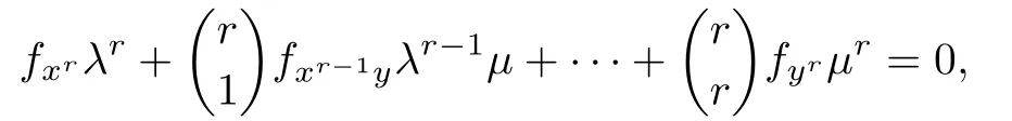
and are counted with multiplicities equal to the multiplicities of the corresponding roots of this equation(see[2]).

A point of multiplicity two or more is said to be singular,and especially,the point of multiplicity two is called a double point.It is evident that a necessary and sufficient condition that a point(a,b)is singular is that

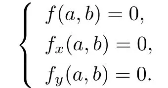
A point P of multiplicity r is ordinary if the r tangents at the point P are distinct. Otherwise P is called non-ordinary.The property of the singular point P of being ordinary or non-ordinary is called the character of P.

By a non-singular curve we mean a curve with no singular points.

We denote f(x,y)in the form

where fk(x,y),0≤k≤d,is a homogeneous polynomial of degree k,fd(x,y)is nonzero and d is called the degree of the plane algebraic curve f(x,y)=0.

Associated with f(x,y)there exists a homogeneous polynomial F(x,y,z)of degree d, the homogenization of f(x,y),

The projective plane algebraic curve D corresponding to C is de fi ned as the set

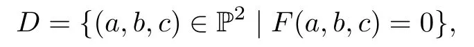
where P2denotes the projective plane.

Every point(a,b)on C corresponds to a point(a,b,1)on D.Every additional point (a,b,0)on D is a point at in fi nity.In other words,the first two coordinates of points at in fi nity are the nontrivial solutions of fd(x,y).So the curve f(x,y)=0 has only finitely many points at in fi nity.We call the points of f(x,y)=0 affine points.

In terms of projective coordinate,the criteria for singular points can be put in a more convenience form.

Proposition 2.1[2]The multiplicity of a pointQofF(x,y,z)=0isrif and only if all the(r−1)-th derivatives ofF(x,y,z),but not all ther-th derivatives,vanish atQ.

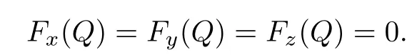
As a corollary of this proposition we see that a point Q of F(x,y,z)=0 is singular if and only if

3 Numerical Procedures and Issues

3.1 Solving the Overdetermined Polynomial Systems

The following proposition shows how to reduce an overdetermined polynomial system to a square system that most of the papers and softwares on continuation method deal with.All the solutions of an overdetermined system appear among the solutions of the corresponding square system,but the converse is not true.

Let n and N be the number of equations and unknown respectively,and n＞N.

Proposition 3.1[14−15]There are nonempty Zariski open dense sets of parametersλi,j∈CN(n−N)orλi,j∈RN(n−N)such that every isolated solution of

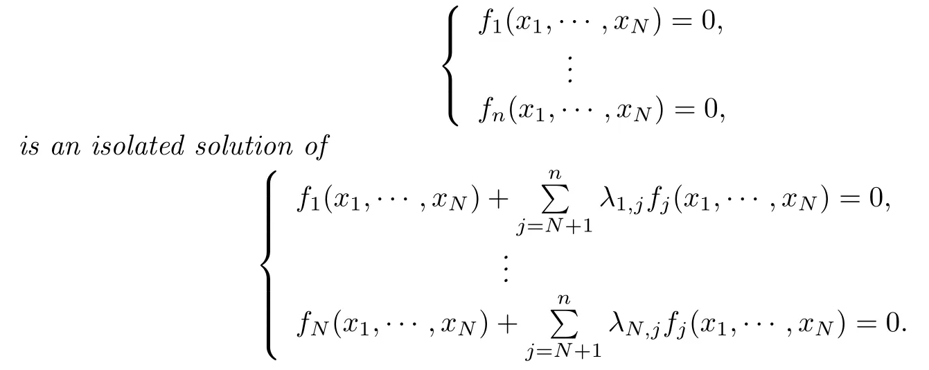
This is just a part of the original proposition and the rest presents the relation between the k≥1 dimensional solution components of the above two systems,however,a theorem in [2]about singular points is that if an irreducible algebraic curve of degree d has multiplicities riat points Pi,then

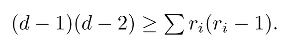
This inequality implies that an irreducible algebraic curve has only finitely many singular points,so the singular point is isolated and the Proposition 3.1 is enough for our demands.

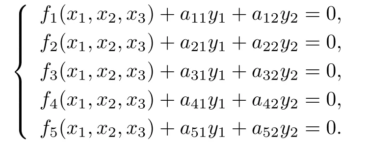
Another technique to deal with the overdetermined polynomial system is to introduce the slack variables.For example,denote X=(x1,x2,x3)and let us consider f(X)= (f1(X),···,f5(X))=0 consisting of fi ve equations in three variables.This technique introduces two new variables y1and y2(so called slack variables)and adds random multiples of these variables to every equation:

The former technique is more attractive for our problem,because fewer equations are left and the dimension of working space is smaller.These two advantages make it more e ff ective than adding the slack variables when solving polynomial systems by homotopy continuation method.

3.2 Remarks for the E ff ect of Tiny Perturbations on the Singular Points

The singular points of algebraic curves are unstable with respect to random perturbations, in other words,tiny perturbations might destroy singular points and their related properties (see[16]).

If we perturb x3−y2=0 with double non-ordinarysingular point(0,0)to x3−y2+ǫx2=0 where ǫ＞0 and is sufficiently small,the singular point is double ordinary singular point (0,0).

The traditional symbolic manipulation may not give the satisfying results for the perturbed algebraic curve.When we give a perturbation 1/1000000 to a monomial coefficient of the algebraic curve with six singular points in Example 4.1 of this paper,the symbolic computation software,Maple,computes only one point by its command“singularities”.

3.3 Computing the Numerical Singular Points,Their Multiplicities and Characters

Given an irreducible plane algebraic curve f(x,y)=0,let its form and homogenous form be as(2.1)and(2.2)respectively,and d be its degree.The numerical procedures to compute the numerical singular points,their multiplicities and characters are as follows.

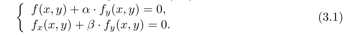
Step 1.Randomization

By Proposition 3.1,choosing the random complex numbers α and β,we add random multiples of the last equation to the first two equations of(1.1),

Step 2.Computing the numerical affine singular points

We solve(3.1)using the polyhedral homotopy continuation method first,and then select the numerical affine singular points from the solutions of(3.1)by evaluating these solutions to f(x,y)respectively.If the value is less than or equal to the given threshold,the corresponding solution is ascertained as a numerical affine singular point.

Step 3.Computing the numerical singular points at in fi nity

The first two coordinates of points at in fi nity are the nontrivial solutions of fd(x,y). Since fd(x,y)is a bivariate homogeneous polynomial of degree d,we can obtain all the numerical points at in fi nity by solving the corresponding univariate polynomial using the method in[13].By Proposition 2.1,we check whether these points at in fi nity are singular by evaluating them to Fx,Fyand Fz,respectively.If all three values are less than or equal to the given threshold,the corresponding point is judged as a numerical singular point at in fi nity.

In the next two steps when we deal with a numerical singular point at in fi nity,the point is transferred to be an affine point by simple linear transformation.

Step 4.Determining the multiplicity

Evaluating the derivatives at a numerical singular point from order equal to 2,if the values of all derivatives of f(x,y)up to and including the(r−1)-th are less than or equal to the given threshold and at least one r-th derivative is greater than the given threshold, the multiplicity of this point will be determined as r.

Step 5.Determining the character

The tangents of f(x,y)=0 at a singular point P of multiplicity r correspond to the roots of

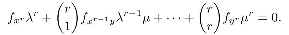
Without a doubt,the coefficients of this polynomial are inexact.The character of the singular point will be determined by if there are multiple roots of this polynomial.

3.4 Numerical Issues about the Procedures of Subsection 3.3

In Step 1,since f is irreducible,f and fxhave no common factors and it holds also for f and fy.So f(x,y)+α·fy(x,y)and fx(x,y)+β·fy(x,y)have no common factors for a probability one set of the coefficients(α,β)of random multiples.All the solutions of(3.1) are isolated and the presented Proposition 3.1 is enough for our demands.

In Step 2,the Jacobian of(3.1)is

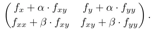
This matrix is singular at a singular point of multiplicity greater than two or almost singular at a numerical singular point of multiplicity greater than two.The numerical techniques of homotopy continuation method could deal with this well.

Homotopy continuation method is a reliable and efficient numerical approach to solving the polynomial systems inCnwhereCis the complex field and is proposed by Garcia and Zangwill[17]in 1979 and Drexler[18]in 1977 independently.The employment of linear homotopies is standard in the early stage.In 1995 Huber and Sturmfels[19]present the polyhedral homotopies based on Bernshtein’s[20]combinatorial root count.For sparse polynomial systems,polyhedral homotopy produces amazing improvements over the classical linear homotopy.The related theories and state of the art techniques can be found in[12, 19,21–22].

Since f(x,y)is not identically zero and has finite degree d,some derivative of order less than or equal to d must be less than or equal to the given threshold at a numerical singular point.Hence Step 4 ends for finitely many numerical singular points.

Univariate polynimials need to be solved in Step 3 and Step 5.Finding the roots of univariate polynomials is one of the fundamental mathematical problems and arises in many scienti fi c and engineering applications.Several methods have been proposed,such as Laguerre’s method,Jenkins-Traub method and the QR algorithm with the companion matrix. However,no one can overcome a barrier of attainable accuracy on an m multiple root(see [23–24]).If there are k1digits machine precision and k2digits coefficients accuracy,the attainable accuracy is min{k1,k2}/m digits.For example,if we use the standard double precision of 16 decimal digits and the accuracy of the polynomial coefficients is 15 digits, only 3 correct digits can be obtained for a root of multiplicity 5.The above standard methods may not compute the multiple roots accurately for univariate polynomials with inexact coefficients,even if the multiprecision is used.A numerical algorithm was presented to calculate multiple roots of univariate polynomials with coefficients possibly being inexact in [13]without extending hardware precision.It is not subject to the accuracy barrier and a lot of numerical experiments have shown its efficiency and robustness.Using this method, we can compute the singular points at in fi nity accurately in Step 3 and the characters of all the singular points can be determined correctly in Step 5.

4 Numerical Results

It is impossible to find exact coefficients of algebraic curves obtained by fi tting or interpolating the experimental data in many fields of science and engineering.As mentioned above, the singular points and their related properties are unstable for the tiny perturbations.In this section some examples are presented to show the efficiency and robustness of numerical procedures in the last section,even if the coefficients of algebraic curves are inexact or perturbed.We also compare some results with those computed by symbolic software Maple. The numerical procedures are implemented in Matlab.

For an irreducible plane algebraic curve with form(2.1)and homogeneous form(2.2),we choose the z=0 as the line at in fi nity,and let(x,y,z)denote a point of F(x,y,z)=0 in the projective plane.(x,y,1)is the point corresponding to a point in the affine plane and (x,y,0)is the point at in fi nity in the following.

For convenience,we use the abbreviations“mult”and“ord”to represent the multiplicity and ordinary in the following tables,respectively.

Example 4.1[25]

There are six double ordinary affine singular points for this curve,i.e.,(−1,−1/2,1), (0,−1,1),(0,0,1),(1,−1/2,1),(−1/2,1,1),(1/2,1,1).Table 4.1 gives the results output by our numerical procedures.Table 4.2 provides the numerical singular points when the coefficient of 51344y5is perturbed to 51344+1/1000000;however,the command“singularities”of Maple gives only one singular point(0,0,1)for the perturbed curve.

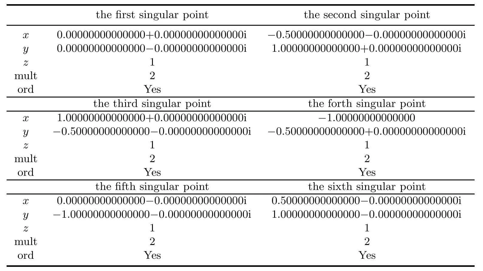
Table 4.1 Singular points,their multiplicities and characters of the curve in Example 4.1

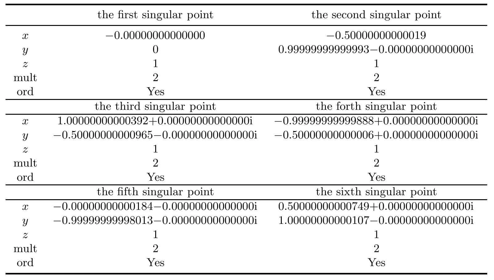
Table 4.2 Singular points,their multiplicities and characters of the curve in Example 4.1 when the coefficient of 51344y5is perturbed to 51344+1/1000000

Example 4.2[10]

There are four double ordinary affine singular points

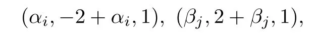
where αi,i=1,2,and βj,j=1,2,are roots of the univariate polynomials

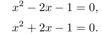
respectively.

Table 4.3 lists the results obtained in our numerical procedures.The singular points are accurate and their multiplicities and characters are correct.

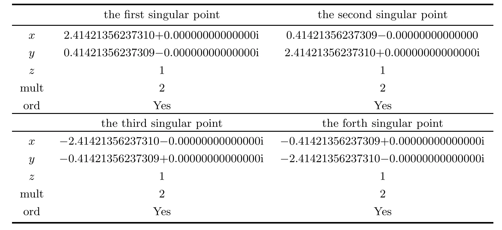
Table 4.3 Singular points,their multiplicities and characters of the curve in Example 4.2

We perturbed the coefficient of 3x5y to 3+1/10000000,3+1/1000000,3+1/100000,3+ 1/10000,3+1/1000 respectively.Tables 4.4–4.8 present our results.Since the multiplicities and characters are all correct,we provide only the numerical singular points and the correct digits are underlined in these fi ve tables.

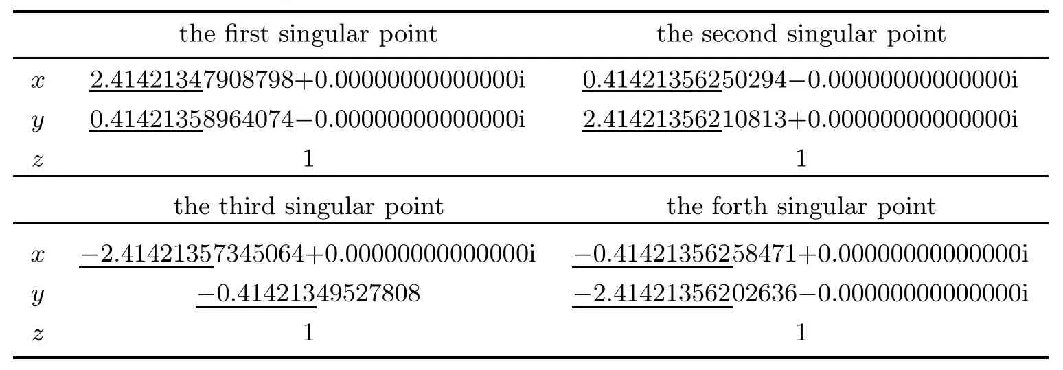
Table 4.4 Singular points in Example 4.2 when the coefficient of 3x5y is perturbed to 3+1/10000000

Table 4.5 Singular points in Example 4.2 when the coefficient of 3x5y is perturbed to 3+1/1000000

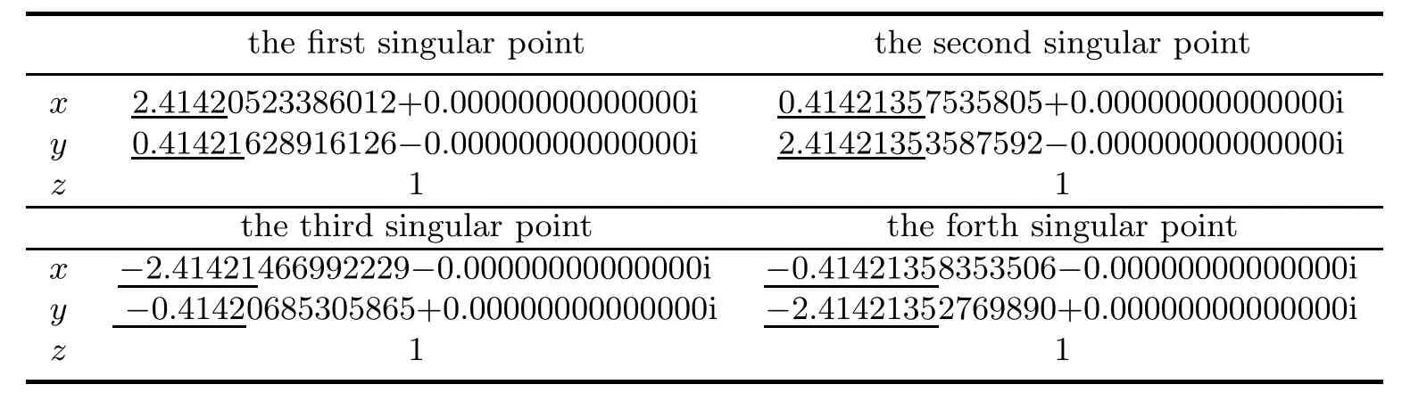
Table 4.6 Singular points in Example 4.2 when the coefficient of 3x5y is perturbed to 3+1/100000

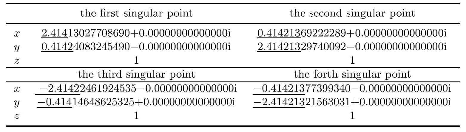
Table 4.7 Singular points in Example 4.2 when the coefficient of 3x5y is perturbed to 3+1/10000

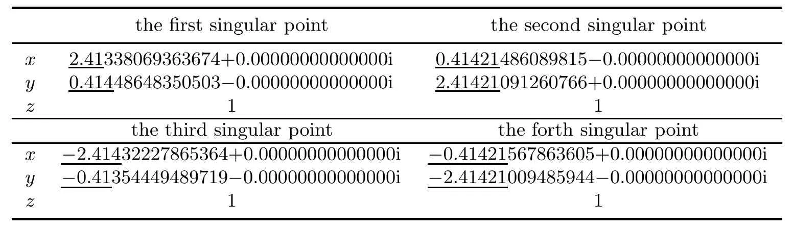
Table 4.8 Singular points in Example 4.2 when the coefficient of 3x5y is perturbed to 3+1/1000

The command“singularities”in Maple provides nothing when the algebraic curve is perturbed in the above fi ve situations.The CPU time of our numerical procedures is almost neglected on the same Lenovo PC with Pentium Dual Core,CPU of 2.5GHZ,memory of 1.99GB.

We usually choose 10−6as the three thresholds in the Step 2,Step 3 and Step 4 of the numerical procedures in Subsection 3.3.When we perturb some coefficients of algebraic curves,the three thresholds may be larger than 10−6.The larger the perturbations are,the larger the thresholds we choose.

Example 4.3[2]

There are no singular points for this algebraic curve.Our numerical procedures output nothing,even if the coefficient of y2x is perturbed to 1+1/100000.

Example 4.4

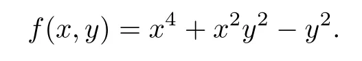
This is a curve with one double non-ordinary affine singular point(0,0,1)and one double ordinary singular point at in fi nity(0,1,0).Table 4.9 presents the results for f(x,y)=0 and Table 4.10 shows the results for the perturbed curve(1+1/1000000)x4+x2y2−y2=0.

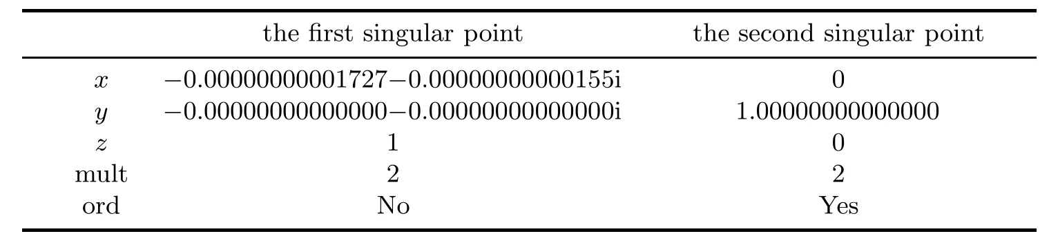
Table 4.9 Singular points,their multiplicities and characters of the curve in Example 4.4

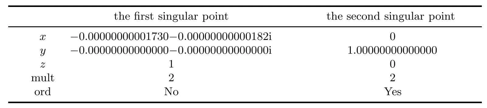
Table 4.10 Singular points,their multiplicities and characters of the curve in Example 4.4 when the coefficient of x4is perturbed to 1+1/1000000

Example 4.5[6]

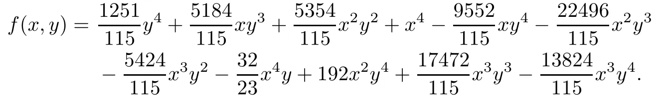
This curve has one ordinary affine singular point(0,0,1)of multiplicity 4,three double ordinary affine singular points(1,1,1),(3/2,1/2,1),(−1/3,1/3,1),one ordinary singular point at in fi nity(0,1,0)of multiplicity 3 and one non-ordinary singular point at in fi nity (1,0,0)of multiplicity 3.

The fractions are truncated in Matlab,so the coefficients of this curve are inexact when we input them,but we still obtain satisfactory results in Table 4.11.

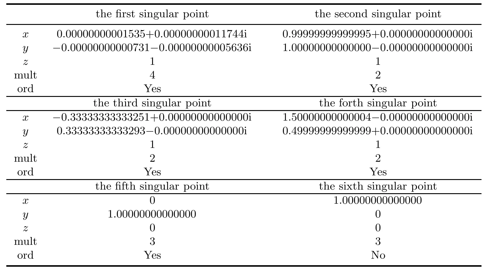
Table 4.11 Singular points,their multiplicities and characters of the curve in Example 4.5

Although non-ordinary is the unstable property for tiny perturbations,the results of Examples 4.4 and 4.5 show that our numerical procedures overcame this barrier and gave the correct character.

5 Concluding Remarks

In cases where the singular points of algebraic curves are all ordinary,the numerical procedures of Section 3 can also determine the genus g of algebraic curves,since

where the summation is over all singular points of multiplicities ri.However,if there exist non-ordinary singular points,the contribution of non-ordinary singular point of multiplicity m to the summation in(5.1)is not simple m(m−1)/2 and in general we need quadratic transformations in[2]to reduce the non-ordinary singular points.

In this paper we present numerical procedures to compute the numerical singular points of irreducible plane algebraic curves and determine their multiplicities and characters.The numerical procedures contain the combined application of homotopy continuation method to solve polynomial systems and calculating the multiple roots of univariate polynomials. The polyhedral homotopy continuation method is the most efficient method to solve the polynomial systems.The method in[13]seems to be the first blackbox to find the roots of univariate polynomials with inexact coefficients using the standard precision arithmetic.

Our numerical procedures can obtain the results accurately and also provide enough correct digits,even if the coefficients of algebraic curves are perturbed.Thus our numerical procedures are not only efficient,but also robust.

AcknowledgementWe thank Li Tien-yien and Zeng Zhong-gang for providing the software packages(HOM4PS-2.0 and MULROOT)on their homepages respectively.

[1]Coolidge J L.A Treatise on Algebraic Plane Curves.New York:Dover,1959.

[2]Walker R J.Algebraic Curves.New York:Springer-Verlag,1978.

[3]Chen F,Wang W,Liu Y.Computing sigular points of plane rational curves.J.Symbolic. Comput.,2008,43:92–117.

[4]Sederberg T W,Anderson D C,Goldman R N.Implicit representation of parametric curves and surfaces.Comput.Vis.Graph.Image Process.,1984,28:72–84.

[5]Abhyankar S S,Bajaj C L.Automatic parameterization of rational curves and surfaces III: Algebraic plane curves.Comput.Aided Geom.Design.,1988,5:309–321.

[6]Sendra J R,Winkler F.Symbolic parametrization of curves.J.Symbolic.Comput.,1991,12: 607–631.

[7]Cox D.Curves,surfaces,and syzygies,topics in algebraic geometry and geometric modeling.Contemp.Math.,2003,334:131–149.

[8]Sun Y,Yu J.Implicitization of parametric curves via Lagrange interpolation.Computing,2006, 77:379–386.

[9]Cox D,Little J,O’Shea D.Ideals,Varieties,and Algorithms:An Introduction to Computational Algebraic Geometry and Commutative Algebra.2nd ed.New York:Springer-Verlag, 1997.

[10]Sakkalis T,Farouki R T.Singular points of algebraic curves.J.Symbolic.Comput.,1990,9: 405–421.

[11]Bajaj C L,Ho ff mann C M,Lynch R E,Hopcroft J E H.Tracing surface intersecitons.Comput. Aided Geom.Design.,1988,5:285–307.

[12]Li T Y.Solving Polynomial Systems by the Homotopy Continuation Method.In:Ciarlet P G. Handbook of Numerical Analysis.vol.XI.Amsterdam:North-Holland,2003.

[13]Zeng Z.Computing multiple roots of inexact polynomials.Math.Comput.,2005,74:869–903.

[14]Sommese A J,Wampler C W.Numerical Algebraic Geometry.In:Renegar J,Shub M,Smale S.The Mathematics of Numerical Analysis:Lectures in Appl.Math.vol.32.Utah:AMS, 1996.

[15]Morgan A P,Sommese A J.Coefficient-parameter polynomial continuation.Appl.Math.Comput.,1989,29:123–160.

[16]Farouki R T,Rajan V T.On the numerical conditions of algebraic curves and surfaces I: implicit equations.Comput.Aided Geom.Design.,1988,5:215–252.

[17]Garcia C B,Zangwill W I.Finding all solutions to polynomial systems and other systems of equations.Math.Program.,1979,16:159–176.

[18]Drexler F J.Eine Methode zur Berechnung samtlicher Losungen von Polynongleichungssystemen.Numer.Math.,1977,29:45–58.

[19]Huber B,Sturmfels B.A Polyhedral method for solving sparse polynomial systems.Math. Comput.,1995,64:1541–1555.

[20]Bernshtein D N.The number of roots of a system of equations.Funct.Anal.Appl.,1975,9: 183–185.

[21]Lee T L,Li T Y,Tsai C H.HOM4PS-2.0:A software package for solving polynomial systems by the polyhedral homotopy continuation method.Computing,2008,83:109–133.

[22]Li T Y,Wang X.The BKK root count in Cn.Math.Comp.,1996,65:161–181.

[23]Pan V Y.Solving polynomial equations:some history and recent progress.SIAM Rev.,1997, 39:187–220.

[24]Igarashi M,Ypma T.Relationships between order and efficiency of a class of methods for multiple zeros of polynomials.J.Comput.Appl.Math.,1984,60:101–113.

[25]Florida State Univ.Department of Math.http://www.math.fsu.edu/hoeij/algcurves.html.

Communicated by Ma Fu-ming

65D99,13D15,14Q05

A

1674-5647(2012)02-0146-13

date:Oct.22,2010.

The NSF(61033012,10801023,11171052,10771028)of China.